 ARIMA models for time series forecasting
Notes
on nonseasonal ARIMA models (pdf file)
Slides on seasonal and
nonseasonal ARIMA models (pdf file)
Introduction
to ARIMA: nonseasonal models
Identifying the order of differencing in an ARIMA model
Identifying the numbers of AR or MA terms in an ARIMA
model
Estimation of ARIMA models
Seasonal differencing in ARIMA models
Seasonal random walk: ARIMA(0,0,0)x(0,1,0)
Seasonal random trend: ARIMA(0,1,0)x(0,1,0)
General seasonal models: ARIMA (0,1,1)x(0,1,1) etc.
Summary of rules for
identifying ARIMA models
ARIMA models with
regressors
The
mathematical structure of ARIMA models (pdf file)
ARIMA models with
regressors
An ARIMA
model can be considered as a special type of regression model--in which the
dependent variable has been stationarized and the independent variables are all
lags of the dependent variable and/or lags of the errors--so it is
straightforward in principle to extend an ARIMA model to incorporate
information provided by leading indicators and other exogenous variables: you
simply add one or more regressors to the forecasting equation.
Alternatively,
you can think of a hybrid ARIMA/regression model as a regression model which
includes a correction for autocorrelated errors. If you have fitted a multiple
regression model and find that its residual ACF and PACF plots display an
identifiable autoregressive or moving-average "signature" (e.g., some
significant pattern of autocorrelations and/or partial autocorrelations at the
first few lags and/or the seasonal lag), then you might wish to consider adding
ARIMA terms (lags of the dependent variable and/or the errors) to the
regression model to eliminate the autocorrelation and further reduce the mean
squared error. To do this, you would just re-fit the regression model as an
ARIMA model with regressors, and you would specify the appropriate AR and/or MA
terms to fit the pattern of autocorrelation you observed in the original
residuals.
Most
high-end forecasting software offers one or more options for combining the
features of ARIMA and multiple regression models. In the Forecasting procedure
in Statgraphics, you can do this by specifying "ARIMA" as the model
type and then hitting the "Regression" button to add regressors.
(Alas, you are limited to 5 additional regressors.) When you add a regressor to
an ARIMA model in Statgraphics, it literally just adds the regressor to the
right-hand-side of the ARIMA forecasting equation. To use a simple case,
suppose you first fit an ARIMA(1,0,1) model with no regressors. Then the
forecasting equation fitted by Statgraphics is:
Ŷt = μ + ϕ1Yt-1 -
θ1et-1
which can
be rewritten as:
Ŷt - ϕ1Yt-1 = μ - θ1et-1
(Note:
this is a standard mathematical form which is often used for ARIMA models. All
terms involving the dependent variable--i.e., all the AR terms and
differences--are collected on the left-hand-side of the equation, while all
terms involving the erorrs--i.e., the MA terms--are collected on the right-hand
side.) Now, if you add a regressor X to the forecasting model, the equation
fitted by Statgraphics is:
Ŷt - ϕ1Yt-1 = μ - θ1et-1 + β(Xt - ϕ1Xt-1)
Thus, the
AR part of the model (and also the differencing transformation, if any) is
applied to the X variable in exactly the same way as it is applied to the Y
variable before X is multiplied by the regression
coefficient. This effectively means that the ARIMA(1,0,1) model is
fitted to the errors of the regression of Y on X (i.e., the series "Y
minus beta X").
How can
you tell if it might be helpful to add a regressor to an ARIMA model? One
approach would be to save the RESIDUALS of the ARIMA model and then look at
their cross-correlations with other potential explanatory variables. For
example, recall that we previously fitted a regression model model to
seasonally adjusted auto sales, in which the LEADIND variable (index of eleven
leading economic indicators) turned out to be slightly significant in addition
to lags of the stationarized sales variable. Perhaps LEADIND would also be
helpful as a regressor in the seasonal ARIMA model we
subsequently fitted to auto sales.
To test
this hypothesis, the RESIDUALS from the ARIMA(0,1,1)x(0,1,1) model fitted to
AUTOSALE were saved. Their cross-correlations with DIFF(LOG(LEADIND)), plotted
in the Descriptive Methods procedure, are as follows:
(A couple
of minor technical points to note here: we have logged and differenced LEADIND
to stationarize it because the RESIDUALS of the ARIMA model are also logged and
differenced--i.e., expressed in units of percentage change. Also, the
Descriptive Methods procedure, like the Forecasting procedure, does not like
variables which begin with too many missing values. Here the missing values at
the beginning of the RESIDUALS variables were replaced by zeroes--typed
in by hand--before running the Descriptive Methods procedure. Actually, the
Forecasting procedure is supposed to automatically draw cross-correlation plots
of the residuals versus other variables, but the graph which is labeled
"Residual Cross-Correlation Plot" merely shows the cross-correlations
of the input variable versus other variables.)
We see that the most significant
cross-correlation is at lag 0, but unfortunately we cannot use that for
forecasting one month ahead. Instead, we must try to exploit the smaller
cross-correlations at lags 1 and/or 2. As a quick test of whether lags of
DIFF(LOG(LEADIND)) are likely to add anything to our ARIMA model, we can use
the Multiple Regression procedure to regress RESIDUALS on lags of
DIFF(LOG(LEADIND)). Here is the result of regressing RESIDUALS on
LAG(DIFF(LOG(LEADIND)),1):
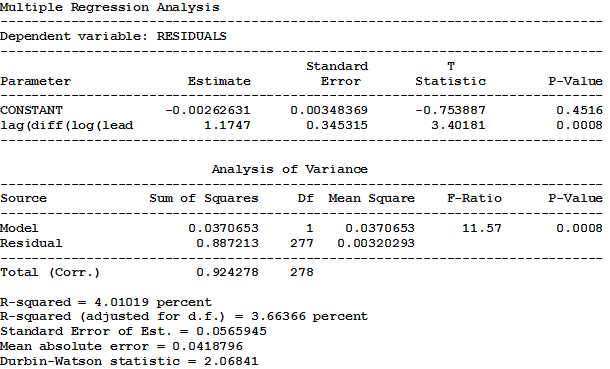
The R-squared value of only 3.66% suggests that not much
improvement is possible. (If two lags of DIFF(LOG(LEADIND)) are used, the
R-squared only increases to 4.06%.) If we return to the ARIMA procedure and add
LAG(DIFF(LOG(LEADIND)),1) as a regressor, we obtain the following model-fitting
results:
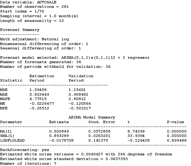
(Minor technical point here: we stored the values of
LAG(DIFF(LOG(LEADIND)),1) in a new column, filled in the two missing values at
the beginning with zeroes, and assigned the new column the name LGDFLGLEAD.) We
see that when a coefficient for the lag of DIFF(LOG(LEADIND)) is estimated simultaneously
with the other parameters of the model, it is even less significant than it
was in the regression model for RESIDUALS. The improvement in the
root-mean-squared error is just too small to be noticeable.
The negative result
we obtained here should not be taken to suggest that regressors will never be
helpful in ARIMA models or other time series models. For example, variables
which measure advertising or price levels or the occurrence of promotional
events are often helpful in augmenting ARIMA models (and exponential smoothing
models) for forecasting sales at the level of the firm or product. Remember
that the variable being analyzed here--nationwide sales at automotive
dealers--is a highly aggregated macroeconomic time series. We have learned by
now that the impact on a macroeconomic variable of events which occurred in earlier
periods (e.g., changes in various economic factors that make up the index
of leading indicators) is often most clearly represented in the prior history
of that variable itself. Hence, lagged values of other macroeconomic time
series may have little to add to a forecasting model which has already fully
exploited the history of the original time series. Leading economic indicators
are often more useful when applied as they are intended--namely as indicators
of turning points in business cycles that may have a bearing on the direction
of longer-term trend projections.