 ARIMA models for time series forecasting
Notes
on nonseasonal ARIMA models (pdf file)
Slides on seasonal and
nonseasonal ARIMA models (pdf file)
Introduction
to ARIMA: nonseasonal models
Identifying the order of differencing in an ARIMA model
Identifying the numbers of AR or MA terms in an ARIMA
model
Estimation of ARIMA models
Seasonal differencing in ARIMA models
Seasonal random
walk: ARIMA(0,0,0)x(0,1,0)
Seasonal random trend: ARIMA(0,1,0)x(0,1,0)
General seasonal models: ARIMA (0,1,1)x(0,1,1) etc.
Summary of rules for identifying ARIMA models
ARIMA models with regressors
The
mathematical structure of ARIMA models (pdf file)
Seasonal random walk
model: ARIMA(0,0,0)x(0,1,0)
If the
seasonal difference (i.e., the season-to-season change) of a time series looks
like stationary noise, this suggests that the mean (constant) forecasting model
should be applied to the seasonal difference. For monthly data, whose seasonal
period is 12, the seasonal difference at period t is Yt-Yt-12.
Applying
the mean model to this series yields the equation:
Ŷt
- Yt-12 = μ
...where μ
is the the mean of the seasonal difference--i.e., the average annual trend
in the data—and Ŷ denotes the
forecast.
Rearranging terms to put Ŷt on the left, we obtain:
Ŷt
= Yt-12 + μ
This
forecasting model will be called the seasonal random walk model, because
it assumes that each season's values form an independent random walk. For
example, the model assumes that September's value this year is a random step
away from September's value last year, October's value this year is a random
step away from October's value last year, etc., and the mean value of every
step is equal to μ:
ŶSep96 = YSep95 + μ
ŶOct96 = YOct95 + μ
and so on.
Notice that the forecast for September '96 ignores all data after September
'95--i.e., it is based entirely on what happened exactly one year ago.
A seasonal
random walk model is a special case of an ARIMA model in which there is one
order of seasonal differencing, a constant term, and no other
parameters--i.e., an "ARIMA(0,0,0)x(0,1,0) model with constant." To
specify a seasonal random walk model in Statgraphics, choose ARIMA as
the model type and use the following settings:
- Differencing:
Nonseasonal Order = 0, Seasonal Order = 1
- AR,
MA, SAR, SMA = 0
- Constant
= ON
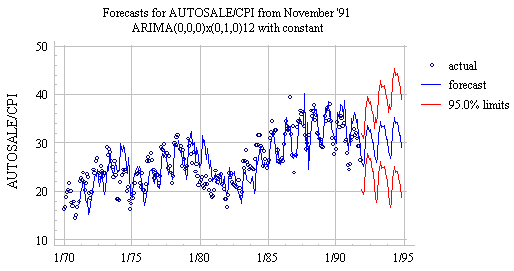
The seasonal difference of the deflated
auto sales data (AUTOSALE/CPI) does not quite look like stationary noise:
it is rather highly correlated. If we fit the seasonal random walk model anyway
(using the ARIMA option in Statgraphics), we obtain the following forecast
plot:

The distinctive
feature of the forecasts produced by this model is that the future seasonal pattern is predicted to have exactly the same
shape as the most recently observed seasonal pattern, and the trend in the
forecasts equals the average trend calculated over the whole history of the
time series. If you look closely at the plot, you will notice that the
model does not respond very quickly to cyclical upturns and downturns in the
data: it is always looking exactly one year behind and assuming that the current
trend equals the average trend, so that when the trend takes an unexpected
upward or downward turn, the forecasts may miss badly in the same direction for
many months in a row. Thus, the one-step-ahead forecast errors typically show
positive autocorrelation. However, the long-term forecasts beyond the end of
the sample appear reasonable insofar as they assume that the average trend in
the past will eventually prevail again in the future.
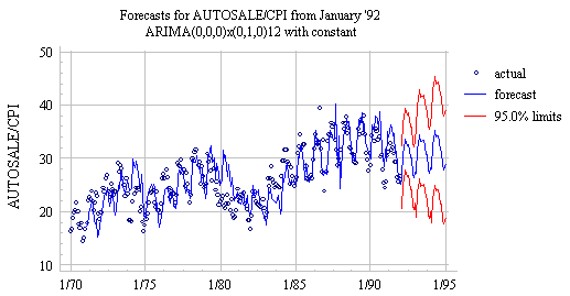
Another
distinctive feature of the seasonal random walk model is that it is relatively
stable in the presence of sudden changes in the data--indeed, it doesn't even
notice them for 12 months! For example, the previous plot shows long-term
forecasts produced from time origin November 1991, at the end of a downward
cycle. A few months later, the data begins to trend upward, but the long-term
forecasts produced by the seasonal random walk model look much the same as
before:

The
positive autocorrelation in the errors of the seasonal random walk model can be
reduced by adding a lag-1 autoregressive ("AR(1)") term to the
forecasting equation. (In Statgraphics, you would do this by additionally
setting AR=1). This yields an "ARIMA(1,0,0)x(0,1,0) model with
constant," and its performance on the deflated auto sales series (from
time origin November 1991) is shown here:

Notice the
much quicker reponse to cyclical turning points. The in-sample RMSE for this
model is only 2.05, versus 2.98 for the seasonal random walk model without the
AR(1) term. (Return to top of page.)
Go to next topic: seasonal random trend model