Using tidyr to create tidy data sets
Description > Easily Tidy Data with ‘spread()’ and ‘gather()’
Functions
A tidy data frame is one where
- Each column is a variable
- Each row is an observatino
- Each value is a cell
As we have seen, tidy data sets can be easily plotted with ggplot2
and manipulated with dplyr. In this notebook, we see how to convert
messy data sets into tidy ones using the verbs gather, spread,
separate, extract, separte_rows and unite.
For more complicated tidying jobs, see the full range of functions in
the `tidyr
documentation <https://cran.r-project.org/web/packages/tidyr/tidyr.pdf>`__.
library(tidyverse)
Data
We will work with a subset of the pilot metadata that we are familiar
with from the dplyr session.
Parsed with column specification:
cols(
  Label = col_character(),
  RNA_sample_num = col_integer(),
  Media = col_character(),
  Strain = col_character(),
  Replicate = col_integer(),
  experiment_person = col_character(),
  libprep_person = col_character(),
  enrichment_method = col_character(),
  RIN = col_double(),
  concentration_fold_difference = col_double(),
  `i7 index` = col_character(),
  `i5 index` = col_character(),
  `i5 primer` = col_character(),
  `i7 primer` = col_character(),
  `library#` = col_integer()
)
Subset the data
| Label | RNA_sample_num | Media | Strain | Replicate | concentration_fold_difference | i7 index | i5 index | i5 primer | i7 primer |
|---|
| 2_MA_C | 2 | YPD | H99 | 2 | 1.34 | ATTACTCG | AGGCTATA | i501 | i701 |
| 9_MA_C | 9 | YPD | mar1d | 3 | 2.23 | ATTACTCG | GCCTCTAT | i502 | i701 |
| 10_MA_C | 10 | YPD | mar1d | 4 | 4.37 | ATTACTCG | AGGATAGG | i503 | i701 |
| 14_MA_C | 14 | TC | H99 | 2 | 1.57 | ATTACTCG | TCAGAGCC | i504 | i701 |
| 15_MA_C | 15 | TC | H99 | 3 | 2.85 | ATTACTCG | CTTCGCCT | i505 | i701 |
| 21_MA_C | 21 | TC | mar1d | 3 | 1.81 | ATTACTCG | TAAGATTA | i506 | i701 |
1. Use gather to combine multiple columns into one
We note thet there are two “index” and “primer” columns - for a tidy
data frame, we probably want to combine them. We cna do this using
gather.
Warm-up
The use of gather can be confusing, so we will start with a toy
example.
| name | jan | feb | mar | apr |
|---|
| ann | 102 | 112 | 123 | 130 |
| bob | 155 | 150 | 147 | 140 |
| charlie | 211 | 211 | 213 | 210 |
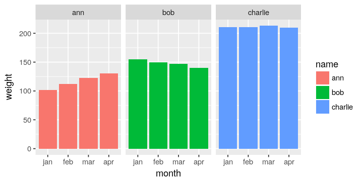
Messy data
In the current form, it is not possible to subgroup by month or to plot
by month easily.
Using gather to creat a new column called weight to store monthly weights
| name | month | weight |
|---|
| ann | jan | 102 |
| bob | jan | 155 |
| charlie | jan | 211 |
| ann | feb | 112 |
| bob | feb | 150 |
| charlie | feb | 211 |
| ann | mar | 123 |
| bob | mar | 147 |
| charlie | mar | 213 |
| ann | apr | 130 |
| bob | apr | 140 |
| charlie | apr | 210 |
To get menth sorted correctly, we make it a factor
| name | month | weight |
|---|
| ann | jan | 102 |
| bob | jan | 155 |
| charlie | jan | 211 |
| ann | feb | 112 |
| bob | feb | 150 |
| charlie | feb | 211 |
| ann | mar | 123 |
| bob | mar | 147 |
| charlie | mar | 213 |
| ann | apr | 130 |
| bob | apr | 140 |
| charlie | apr | 210 |
Now we can easily work wtih the tidy data set
| month | min | max | mean |
|---|
| jan | 102 | 211 | 156.0000 |
| feb | 112 | 211 | 157.6667 |
| mar | 123 | 213 | 161.0000 |
| apr | 130 | 210 | 160.0000 |
Data type cannot be displayed:
2. Use spread to convert one column into multiple
We can undo gather with spread. This is less commonly used than
gather.
| Label | index | sequence |
|---|
| 2_MA_C | i7 index | ATTACTCG |
| 9_MA_C | i7 index | ATTACTCG |
| 10_MA_C | i7 index | ATTACTCG |
| 14_MA_C | i7 index | ATTACTCG |
| 15_MA_C | i7 index | ATTACTCG |
| 21_MA_C | i7 index | ATTACTCG |
| Label | i5 index | i7 index |
|---|
| 1_MA_J | AGGCTATA | CGCTCATT |
| 1_RZ_J | AGGCTATA | GAGATTCC |
| 10_MA_C | AGGATAGG | ATTACTCG |
| 10_RZ_C | AGGATAGG | TCCGGAGA |
| 11_MA_J | AGGATAGG | CGCTCATT |
| 11_RZ_J | AGGATAGG | GAGATTCC |
3. Use separate to split a single column containing multiple values
The label column actually contains three pieces of informaiton separated
by underscores - a sample number, the RNA enrichment methd, and code for
the person presenting the sample. Assuuming that we do not have this
informatio nduplicate in other columns, it woujld be tricky to compare,
say, results by the sampling method.
The separate function is designed to address this problem.
| Label | concentration_fold_difference |
|---|
| 2_MA_C | 1.34 |
| 9_MA_C | 2.23 |
| 10_MA_C | 4.37 |
| sample_num | enrichment | person | concentration_fold_difference |
|---|
| 2 | MA | C | 1.34 |
| 9 | MA | C | 2.23 |
| 10 | MA | C | 4.37 |
Here is a summary of the data.
| person | enrichment | n | concentration_fold_difference |
|---|
| C | MA | 24 | 2.3675 |
| C | RZ | 24 | 2.3675 |
| C | TOT | 3 | 1.3400 |
| J | MA | 24 | 3.4350 |
| J | RZ | 24 | 3.4350 |
| J | TOT | 3 | 1.9800 |
| P | MA | 24 | 3.0800 |
| P | RZ | 24 | 3.0800 |
| P | TOT | 3 | 2.0500 |
4. Use unite to craate a single variable from multiple columns
Sometimes we want to do the opposite and combine multiple columns into a
single column. Use unite to do this.
| sample_num | enrichment | person | concentration_fold_difference |
|---|
| 2 | MA | C | 1.34 |
| 9 | MA | C | 2.23 |
| 10 | MA | C | 4.37 |
| 14 | MA | C | 1.57 |
| 15 | MA | C | 2.85 |
| 21 | MA | C | 1.81 |
| Label | concentration_fold_difference |
|---|
| 2_MA_C | 1.34 |
| 9_MA_C | 2.23 |
| 10_MA_C | 4.37 |
| 14_MA_C | 1.57 |
| 15_MA_C | 2.85 |
| 21_MA_C | 1.81 |
Sometiems there is no simple delimiter between parts of a value. In such
cases, we may need to use reuglar expressions to extract parts from a
string.
| Label | concentration_fold_difference |
|---|
| 2MAC | 1.34 |
| 9MAC | 2.23 |
| 10MAC | 4.37 |
| 14MAC | 1.57 |
| 15MAC | 2.85 |
| 21MAC | 1.81 |
The regular expression consists of 3 capture groups in parentheses that
will form the new columns.
'([0-9]+)(.*)(.$)'
where
- Capture group 1
[0-9]+ means match one or more + of any
digits [0-9]
- Capture group 2
.* means match zero or more * of any
character .
- Capture gorup 3
.$ means match any character . at the end
$
| sample_num | enrichment | person | concentration_fold_difference |
|---|
| 2 | MA | C | 1.34 |
| 9 | MA | C | 2.23 |
| 10 | MA | C | 4.37 |
| 14 | MA | C | 1.57 |
| 15 | MA | C | 2.85 |
| 21 | MA | C | 1.81 |
Using separate_rows rows when multiple values are in a single cell.
Very occassionally, we find data sets where multiple values are stored
in a single cell. We will make up and exmple here as this does not occur
in the metadata data set.
| Label | primer |
|---|
| 1_MA_J | AGGCTATA,CGCTCATT |
| 1_RZ_J | AGGCTATA,GAGATTCC |
| 10_MA_C | AGGATAGG,ATTACTCG |
| 10_RZ_C | AGGATAGG,TCCGGAGA |
| 11_MA_J | AGGATAGG,CGCTCATT |
| 11_RZ_J | AGGATAGG,GAGATTCC |
| Label | primer |
|---|
| 1_MA_J | AGGCTATA |
| 1_MA_J | CGCTCATT |
| 1_RZ_J | AGGCTATA |
| 1_RZ_J | GAGATTCC |
| 10_MA_C | AGGATAGG |
| 10_MA_C | ATTACTCG |
Challenge exercise
Let’s look at the index and primer columne more closely. It seems that
the index and primer values are linked and are just different ways of
labeling the same thing. So we really should be have columns like this
| primer_type |
code |
seq |
|---|
| i5 |
i501 |
AGGCTATA |
| i5 |
i502 |
GCCTCTAT |
| i7 |
i701 |
ATTACTCG |
| i7 |
i702 |
TCCGGAGA |
We can do this by combining the operatios we have seen above.
| Label | RNA_sample_num | Media | Strain | Replicate | concentration_fold_difference | primer_type | code | seq |
|---|
| 2_MA_C | 2 | YPD | H99 | 2 | 1.34 | i5 | 01 | AGGCTATA |
| 2_RZ_C | 2 | YPD | H99 | 2 | 1.34 | i5 | 01 | AGGCTATA |
| 2_TOT_C | 2 | YPD | H99 | 2 | 1.34 | i5 | 01 | AGGCTATA |
| 1_MA_J | 1 | YPD | H99 | 1 | 3.64 | i5 | 01 | AGGCTATA |
| 1_RZ_J | 1 | YPD | H99 | 1 | 3.64 | i5 | 01 | AGGCTATA |
| 4_MA_P | 4 | YPD | H99 | 4 | 2.05 | i5 | 01 | AGGCTATA |
| 4_RZ_P | 4 | YPD | H99 | 4 | 2.05 | i5 | 01 | AGGCTATA |
| 9_MA_C | 9 | YPD | mar1d | 3 | 2.23 | i5 | 02 | GCCTCTAT |
| 9_RZ_C | 9 | YPD | mar1d | 3 | 2.23 | i5 | 02 | GCCTCTAT |
| 3_MA_J | 3 | YPD | H99 | 3 | 1.98 | i5 | 02 | GCCTCTAT |