Mathematical and Physical Foundations¶

Introduction¶

Daphne is a software system for creating and running the simulations of multi-cellular systems. This document provides guidance on the mathematics behind the simulation system.

Daphne is built on the generic processes of Newtonian mechanics, and generalized chemical kinetics, as well as a small number of cell biology-specific constructs. That is, for example, any entity that has a position changes its position in accordance with Newton’s laws. Forces arise in the mechanical interactions of cells and as a result of molecular interactions and molecular conformational changes. Collections of entities, typically cells or molecules, can be treated as continua and described by their concentration or density fields as well as by a lists of individual positions (and velocities). These fields obey kinetic equations derived from mass-action kinetics.

Molecular concentrations and related quantities are often modeled as continuous scalar fields in space that evolve continuously in time in response to physical processes, such as reaction and diffusion. Obtaining analytical solutions for these quantities at all spatial and time points is generally not possible for complex biological systems, and numerical techniques must be used to obtain approximations of the dynamical behavior of the system. Generally, techniques for approximating the temporal and spatial aspects of the problem are implemented independently.

Currently in Daphne, we implement two types of approximations for the spatial dependence of the system, moment-expansion and discrete, each with a distinct scalar field representation. In the moment-expansion scalar field representation, the spatial dependence of a quantity is represented by an infinite series expansion, with each successive term accounting for the next (higher-order) moment (of the spatial distribution) of the system. The spatial accuracy of the moment-expansion approximation is determined by the number of terms in the infinite series that are retained for calculations. With this numerical approach, the quantities of interest are still functions of continuous spatial variables. Currently, Daphne utilizes two-term moment-expansion fields to describe scalar fields in cells. The advantage of this representation is that it provides computational efficiency while still providing information about the spatial distribution, or polarity, of a scalar field, through the second (dipole) term. This polarity is crucial for modeling cellular processes, such as chemotaxis.

In contrast, the discretized numerical approach seeks solutions to the dynamical equations at only a (finite) set of discrete spatial points in the space of interest, and the values of quantities at intermediate spatial points are approximated through interpolation of the solutions at the discrete (lattice) points. The spatial accuracy of the discretized approximation is determined by the density of discrete points and the size of the neighborhood (number of nearest neighbors) that is used to approximate the equations.

Moment expansion scalar fields¶

We can represent a scalar field \(c({\bf v})\) as a moment expansion

(1)\[ c({\bf v}) = c^{(0)} + c^{(1)}_{i} v_i + c^{(2)}_{ij} v_i v_j +c^{(3)}_{ijk} v_i v_j v_k + \ldots\]

where \({\bf v} \in \mathbb{R}^3\) and summation over indices is assumed. To first order,

(2)\[\begin{split} c({\bf v}) & \approx & c^{(0)} + {\bf c}^{(1)} \cdot {\bf v}.\end{split}\]

Notes:

1. The definition (2) of the second-order moment-expansion is also applicable to scalar fields defined on surfaces \(\mathbb{R}^2\) in \(\mathbb{R}^3\).

Moment-expansions of scalar fields defined on surfaces are defined in terms of vectors

in the embedding space (\({\bf v}\), \({\bf c}^{(1)}\) \(\in \mathbb{R}^3\)), even though the surface is inherently of lower order.

However, the calculation and units of the coefficients \(c^{(0)}\) and \({\bf c}^{(1)}\)

are dependent upon the manifold (eg, ball, sphere) on which the scalar field is defined.

The zeroth moment \(c^{(0)}\) is the mean value of the scalar field.
The first moment \({\bf c}^{(1)}\) is
1. the weighted mean position
2. analogous to the center-of-mass in physics

4. The coefficients in the moment-expansion (2) are analogous to moments in statistics.

In this sense, the scalar field is analogous to the probability density,

although it may not be normalized which is why \(c^{(0)}\) is not necessarily equal to one.

The first moment \({\bf c}^{(1)}\) is the mean (spatial) position.

Mathematical operations¶

Addition¶

To first order, the moment-expansion representation of the scalar field resulting from addition of two scalar fields is given by

(3)\[\begin{split}\boxed{ \renewcommand{\arraystretch}{1.0} \begin{array}{rcl} c({\bf v}) &=& a({\bf v}) + b({\bf v}) = c^{(0)} + {\bf c}^{(1)} \cdot {\bf v} \\ c^{(0)} &=& a^{(0)}+ b^{(0)} \\ {\bf c}^{(1)} &=& {\bf a}^{(1)} + {\bf b}^{(1)} \end{array} }\end{split}\]

Multiplication¶

To first order, the moment-expansion representation of the scalar field resulting from multiplication of two scalar fields is

(4)\[\begin{split} c({\bf v}) & = & a({\bf v}) b({\bf v}) = c^{(0)} + {\bf c}^{(1)} \cdot {\bf v} = \left(a^{(0)} + {\bf a}^{(1)} \cdot {\bf v} \right) \left( b^{(0)} + {\bf b}^{(1)} \cdot {\bf v} \right)\end{split}\]

(5)\[\begin{split}\boxed{ \renewcommand{\arraystretch}{1.5} \begin{array}{rcl} c^{(0)} &=& a^{(0)} b^{(0)} \\ {\bf c}^{(1)} &=& a^{(0)} {\bf b}^{(1)} + b^{(0)} {\bf a}^{(1)} \end{array} }\end{split}\]

Application to a sphere¶

We have a spherical surface \(S\) of radius \(\rho\) centered at the origin with a scalar field \(c({\bf x})\) defined on the surface, where \({\bf x}\) is a vector pointing from the origin to the point \((x,y,z)\) on the sphere surface.

The moment-expansion representation of the scalar field \(c({\bf x})\) on the sphere is given by

(6)\[\begin{split}c({\bf x}) & = & c^{(0)} + {\bf c}^{(1)} \cdot {\bf x} ,\end{split}\]

where the coefficients \(c^{(0)} \in \mathbb{R}\) and \({\bf c}^{(1)} \in \mathbb{R}^3\) are given by the moment equations

(7)\[\begin{split} ^{(0)} & = & \frac{1}{4\pi \rho^2} \int_{S} dS\; c({\bf x}) \\ {\bf c^{(1)}} & = & \frac{3}{4\pi \rho^4} \int_{S} dS\; c({\bf x}) \; {\bf x} ,\end{split}\]

and have the units \(\left[ c \right]\) and \(\frac{[c]}{L}\), respectively.

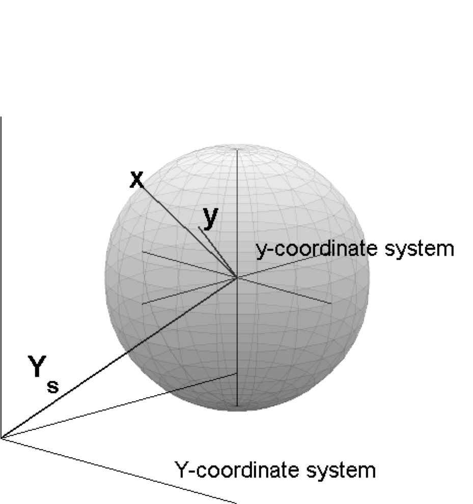
Figure 1: The global ECS \(Y\)-coordinate system and the local \(y\)-coordinate system of the sphere. The sphere is located at position \({\bf Y_s}\). The vector \({\bf x}\) refers to a point on the surface of the sphere. The vector \({\bf y}\) refers to a point in, or on the surface of, the sphere.

Sphere gradient¶

Application of the gradient operator \(\nabla f = \frac{\partial f}{\partial x} \hat{x} + \frac{\partial f}{\partial y} \hat{y} + \frac{\partial f}{\partial z} \hat{z}\) to a moment-expansion scalar field on the sphere gives, to first order,

(8)\[\begin{split}\begin{array}{rcl} {\bf \nabla} c (\rho {\bf \hat{u}}) & \approx & {\bf \nabla} \left( c^{(0)} + \rho {\bf c^{(1)}}\cdot {\bf \hat{u} } \right) = \rho {\bf \nabla}\left( {\bf c^{(1)}}\cdot {\bf \hat{u}} \right) , \end{array}\end{split}\]

where \({\bf \hat{u}} = u_x\hat{x} + u_y \hat{y} + u_z \hat{z} = \frac{ x \hat{x} + y \hat{y} + z \hat{z} }{ \left( x^2 + y^2 + z^2 \right)^{\frac{1}{2}} }\) is the unit vector from the origin in the direction of the point \((x,y,z)\) on the sphere.

Using the identities (121) and (134) and the fact that \({\bf c^{(1)}}\) is a constant vector, the right-hand side of (8) can be written as

(9)\[\begin{split}\begin{array}{rcl} \rho {\bf \nabla}\left( {\bf c^{(1)}} \cdot {\bf \hat{u}} \right) & = & \rho \left( {\bf c^{(1)}} \cdot {\bf \nabla} \right) {\bf \hat{u}} \end{array}\end{split}\]

The right-hand side of (9) has vector components \(\left( \sum_{i=1}^{3} c^{(1)}_i \partial_i \right) u_j\) with \(j=1,2,3\), which produce the following terms for the \(x\) -component (\(j=1\) case)

(10)\[\begin{split}\begin{array}{rcl} \frac{\partial }{\partial x} \frac{ x \hat{x} }{ \left( x^2 + y^2 + z^2 \right)^{\frac{1}{2}} } & = & - \frac{ x^2 \hat{x} }{ \left( x^2 + y^2 + z^2 \right)^{\frac{3}{2}} } + \frac{ \hat{x} }{ \left( x^2 + y^2 + z^2 \right)^{\frac{1}{2}} } \\ % \frac{\partial }{\partial y} \frac{ x \hat{x} }{ \left( x^2 + y^2 + z^2 \right)^{\frac{1}{2}} } & = & - \frac{ x y \hat{x} }{ \left( x^2 + y^2 + z^2 \right)^{\frac{3}{2}} } \\ % \frac{\partial }{\partial z} \frac{ x \hat{x} }{ \left( x^2 + y^2 + z^2 \right)^{\frac{1}{2}} } & = & - \frac{ x z \hat{x} }{ \left( x^2 + y^2 + z^2 \right)^{\frac{3}{2}} } \end{array}\end{split}\]

Gathering the terms in (10) and generalizing to the \(y\)- and \(z\)-components gives

(11)\[\begin{split}\begin{array}{rcl} \left( \sum_{i=1}^{3} c^{(1)}_i \partial_i \right) \frac{ x \hat{x} }{ \left( x^2 + y^2 + z^2 \right)^{\frac{1}{2}} } & = & - \frac{ x \left( c^{(1)}_x x + c^{(1)}_y y + c^{(1)}_z z \right) \hat{x} }{ \left( x^2 + y^2 + z^2 \right)^{\frac{3}{2}} } + \frac{ c^{(1)}_x \hat{x} }{ \left( x^2 + y^2 + z^2 \right)^{\frac{1}{2}} } \\ & = & - \frac{1}{\rho} \left( c^{(1)}_x u_x + c^{(1)}_y u_y + c^{(1)}_z u_z \right) u_x \hat{x} + \frac{1}{\rho} c^{(1)}_x \hat{x} \\ & = & \frac{1}{\rho} c^{(1)}_x \hat{x} - \frac{1}{\rho} \left( {\bf c^{(1)}} \cdot {\bf \hat{u}} \right) x \hat{x} \\ % \left( \sum_{i=1}^{3} c^{(1)}_i \partial_i \right) \frac{ y \hat{y} }{ \left( x^2 + y^2 + z^2 \right)^{\frac{1}{2}} } % & = & - \frac{ y \left( c^{(1)}_x x + c^{(1)}_y y + c^{(1)}_z z \right) \hat{y} }{ \left( x^2 + y^2 + z^2 \right)^{\frac{3}{2}} } % + \frac{ c^{(1)}_y \hat{y} }{ \left( x^2 + y^2 + z^2 \right)^{\frac{1}{2}} } \\ % & = & - \frac{1}{\rho} \left( c^{(1)}_x u_x + c^{(1)}_y u_y + c^{(1)}_z u_z \right) u_y \hat{y} % + \frac{1}{\rho} c^{(1)}_y \hat{y} \\ & = & \frac{1}{\rho} c^{(1)}_y \hat{y} - \frac{1}{\rho} \left( {\bf c^{(1)}} \cdot {\bf \hat{u}} \right) y \hat{y} \\ % \left( \sum_{i=1}^{3} c^{(1)}_i \partial_i \right) \frac{ z \hat{z} }{ \left( x^2 + y^2 + z^2 \right)^{\frac{1}{2}} } % & = & - \frac{ z \left( c^{(1)}_x x + c^{(1)}_y y + c^{(1)}_z z \right) \hat{y} }{ \left( x^2 + y^2 + z^2 \right)^{\frac{3}{2}} } % + \frac{ c^{(1)}_z \hat{z} }{ \left( x^2 + y^2 + z^2 \right)^{\frac{1}{2}} } % & = & - \frac{1}{\rho} \left( c^{(1)}_x u_x + c^{(1)}_y u_y + c^{(1)}_z u_z \right) u_z \hat{z} % + \frac{1}{\rho} c^{(1)}_z \hat{z} & = & \frac{1}{\rho} c^{(1)}_z \hat{z} - \frac{1}{\rho} \left( {\bf c^{(1)}} \cdot {\bf \hat{u}} \right) z \hat{z} \end{array}\end{split}\]

and

(12)\[\begin{split}\begin{array}{rcl} {\bf \nabla}\left( {\bf c^{(1)}}\cdot {\bf \hat{u}} \right) & = & \frac{1}{\rho} {\bf c^{(1)}} - \frac{1}{\rho} \left( {\bf c^{(1)}} \cdot {\bf \hat{u}} \right) {\bf \hat{u}} \end{array}\end{split}\]

Combining (8) and (12) gives the first-order moment expansion of the gradient of a scalar field on the sphere

(13)\[\begin{split}\boxed{ \renewcommand{\arraystretch}{2.0} \begin{array}{rcl} {\bf \nabla} c ({\bf \hat{u}}) %& = & \rho {\bf \nabla}\left( {\bf c^{(1)}}\cdot {\bf u} \right) & = & {\bf c^{(1)}} - \left( {\bf c^{(1)}} \cdot {\bf \hat{u}} \right) {\bf \hat{u}} . \end{array} }\end{split}\]

Sphere laplacian¶

The result of the application of the Laplacian operator to a scalar field on the sphere can be (to first order) resolved into it’s first two moment-expansion components

(14)\[\begin{array}{rcl} \nabla^2 c({\bf x}) \approx l^{(0)} + {\bf l^{(1)}} \cdot {\bf x}, \end{array}\]

with units of \(\frac{[c]}{L^2}\) and \(\frac{[c]}{L^3}\) for the coefficients \(l^{(0)}\) and \({\bf l^{(1)}}\) , respectively.

Zeroth moment. The zeroth moment of the laplacian operator acting on the scalar field is given by

(15)\[\begin{split}\begin{array}{rcl} l^{(0)} & = & \frac{1}{4\pi \rho^2} \int_{S} dS\, \nabla^2 c({\bf x}) = \frac{1}{4\pi \rho^2} \int_{S} dS\, \nabla^2 c(\rho {\bf \hat{u}}) \end{array}\end{split}\]

where \({\bf \hat{u}} =u_x\hat{x} + u_y\hat{y} +u_z \hat{z} = \frac{ x \hat{x} + y \hat{y} + z \hat{z} }{ \left( x^2 + y^2 + z^2 \right)^{\frac{1}{2}} }\) is the unit vector from the origin in the direction of the point \((x,y,z)\) on the sphere.

Using the results in Section Laplacian of scalar field integrated over sphere surface, \(\int_{S} dS\, \nabla^2 c({\bf x})= 0\) and

(16)\[\boxed{ \renewcommand{\arraystretch}{1.0} \begin{array}{rcl} l^{(0)} = 0 \end{array} }\]

First moment. The first moment of the laplacian operator acting on the scalar field is given by

(17)\[\begin{split}\begin{array}{rcl} {\bf l^{(1)}} & = & \frac{3}{4\pi \rho^4} \int_{S} dS\, \nabla^2 c( {\bf x}) \; {\bf x} = \frac{3}{4\pi \rho^3} \int_{S} dS\, \nabla^2 c(\rho {\bf \hat{u}}) \; {\bf \hat{u}}, \end{array}\end{split}\]

where \({\bf \hat{u}} =u_x\hat{x} + u_y\hat{y} +u_z \hat{z} = \frac{ x \hat{x} + y \hat{y} + z \hat{z} }{ \left( x^2 + y^2 + z^2 \right)^{\frac{1}{2}} }\) is the unit vector from the origin in the direction of the point \((x,y,z)\) on the sphere.

Using the identity (138) we get

(18)\[\begin{split}\begin{array}{rcl} \frac{3}{4\pi \rho^3} \int_{S} dS\, \nabla^2 c(\rho {\bf \hat{u}}) \; {\bf \hat{u}} & = & \frac{3}{4\pi \rho^3} \int_{S} dS\, \left[ \nabla \cdot \left( \nabla c \; {\bf \hat{u}} \right) + \frac{1}{\rho} \left( \nabla c \cdot {\bf \hat{u}} \right) {\bf \hat{u}} - \frac{1}{\rho} \left( \nabla c \right) \right] . \end{array}\end{split}\]

We will apply the first order gradient expansion (13), \({\bf \nabla} c ({\bf \hat{u}}) = {\bf c^{(1)}} - \left( {\bf c^{(1)}} \cdot {\bf \hat{u}} \right) {\bf \hat{u}}, \;\) to the terms on the right-hand side of the above equation and keep only first order terms.

First term.

(19)\[\begin{array}{rcl} \frac{3}{4\pi \rho^3} \int_{S} dS\, \nabla \cdot \left( \nabla c(\rho {\bf \hat{u}}) {\bf \hat{u}} \right) = \frac{3}{4\pi \rho^3} \int_{S} dS\, \left[ \nabla \cdot \left( {\bf c^{(1)}} {\bf \hat{u}} \right) - \nabla \cdot \left( \left( {\bf c^{(1)}} \cdot {\bf \hat{u}} \right) {\bf \hat{u}} {\bf \hat{u}} \right) \right] = 0 \end{array}\]

Second term.

(20)\[\begin{array}{rcl} \left( \nabla c \cdot {\bf \hat{u}} \right) {\bf \hat{u}} = \left( {\bf c^{(1)}} \cdot {\bf \hat{u}} \right) {\bf \hat{u}} - \left( \left( {\bf c^{(1)}} \cdot {\bf \hat{u}} \right) {\bf \hat{u}} \cdot {\bf \hat{u}} \right) {\bf \hat{u}} = \left( {\bf c^{(1)}} \cdot {\bf \hat{u}} \right) {\bf \hat{u}} - \left( {\bf c^{(1)}} \cdot {\bf \hat{u}} \right) {\bf \hat{u}} = 0 \end{array}\]

Third term.

(21)\[\begin{split}\begin{array}{rcl} \frac{3}{4\pi \rho^4} \int_{S} dS\, \nabla c & = & \frac{3}{4\pi \rho^4} \int_{S} dS\, \left[ {\bf c^{(1)}} - \left( {\bf c^{(1)}} \cdot {\bf \hat{u}} \right) {\bf \hat{u}} \right] \\ & = & \frac{3}{4\pi \rho^4} {\bf c^{(1)}} 4 \pi \rho^2 - \frac{3}{4\pi \rho^4} \int_{S} dS\, \left( {\bf c^{(1)}} \cdot {\bf \hat{u}} \right) {\bf \hat{u}} \\ & = & \frac{3}{\rho^2} {\bf c^{(1)}} - \frac{3}{4\pi \rho^4} \int_{S} dS\, \left( {\bf c^{(1)}} \cdot {\bf \hat{u}} \right) {\bf \hat{u}} \end{array}\end{split}\]

Applying the identity (143), \(\int_{S} dS \;\; \left( {\bf a} \cdot {\bf\hat{u}} \right) \hat{\bf u} = \frac{4 \pi}{3} \rho^2 {\bf a}, \;\,\)

gives

(22)\[\begin{split}\begin{array}{rcl} \frac{3}{4\pi \rho^4} \int_{S} dS\, \nabla c & = & \frac{2}{\rho^2} {\bf c^{(1)}} \end{array}\end{split}\]

In summary, the moment-expansion representation of the laplacian applied to a scalar field defined on the sphere is given, to first order, by

(23)\[\begin{split}\boxed{ \renewcommand{\arraystretch}{2.0} \begin{array}{rcl} \nabla^2 c({\bf x}) & \approx & l^{(0)} + {\bf l^{(1)} } \cdot {\bf x} \\ l^{(0)} & = & 0\\ {\bf l^{(1)} } & = & -\frac{2}{\rho^2} {\bf c^{(1)}}. \end{array} }\end{split}\]

Sphere diffusion equation¶

The diffusion equation is

(24)\[\renewcommand{\arraystretch}{1.0} \begin{array}{rcl} \frac{\partial c({\bf x})}{\partial t} = \zeta\, \nabla^2 c({\bf x}) , \end{array}\]

where \(\zeta\) is the diffusion coefficient. Applying (23) to (24) and keeping first-order terms gives

(25)\[\begin{split}\renewcommand{\arraystretch}{2.0} \begin{array}{rcl} \frac{\partial c({\bf x})}{\partial t} & \approx & \zeta \left( l^{(0)} + {\bf l^{(1)}} \cdot {\bf x} \right) = - \frac{2}{\rho^2}\, \zeta\; {\bf c^{(1)}} \cdot {\bf x}. \end{array}\end{split}\]

Restriction to tiny sphere¶

Consider a 3D volume \(V\) with coordinate system \({\bf Y}\), a scalar field \(F({\bf Y})\) defined in \(V\), and a spherical surface \(S\) with radius \(\rho\) located at position (sphere center) \({\bf Y_s}\) in \(V\).

The value of the scalar field at the surface of the sphere can be approximated by a moment-expansion scalar field \(f({\bf x})\) defined with respect to a local coordinate system \({\bf x}\) at \({\bf Y_s}\)

(26)\[\begin{split}\renewcommand{\arraystretch}{1.0} \begin{array}{rcl} F({\bf Y(x)}) = f({\bf x}) & \approx & f^{(0)} + {\bf f^{(1)}} \cdot {\bf x}. \end{array}\end{split}\]

In the limit of that the radius of the sphere is very small, we can approximate that the scalar field \(F({\bf Y})\) is unperturbed by the presence of the sphere. Then using the Taylor expansion,

\[F({\bf Y_s+ x} ) \approx F({\bf Y_s}) + \nabla F({\bf Y_s}) \cdot {\bf x},\]

in the definition for the zeroth moment (7) gives

(27)\[\begin{split}\renewcommand{\arraystretch}{1.0} \begin{array}{rcl} f^{(0)} & = & \frac{1}{4\pi \rho^2} \int_{S} dS\; F({\bf Y_s+ x}) \approx \frac{1}{4\pi \rho^2} \int_{S} dS\; \left[ F({\bf Y_s}) + \nabla F({\bf Y_s}) \cdot {\bf x} \right] = F({\bf Y_s}) . \end{array}\end{split}\]

Similarly, using the above Taylor expansion, as well as relation (143) in the definition of the first moment (7) gives

(28)\[\begin{split}\renewcommand{\arraystretch}{2.0} \begin{array}{rcl} {\bf f^{(1)}} & = & \frac{3}{4\pi \rho^4} \int_{S} dS\; F({\bf Y_s+ x}) {\bf x} \\ & \approx & \frac{3}{4\pi \rho^4} \int_{S} dS\; \left[ F({\bf Y_s}) + \nabla F({\bf Y_s}) \cdot {\bf x} \right] {\bf x} \\ %& = & \frac{3}{4\pi \rho^4} \int_{S} dS\; \nabla F({\bf Y_s}) \cdot {\bf x} \, {\bf x} \\ & = & \frac{3}{4\pi \rho^2} \int_{S} dS\; \nabla F({\bf Y_c}) \cdot {\bf \hat{x}} \, {\bf \hat{x}} \\ %& = & \frac{3}{4\pi \rho^2} \frac{4\pi}{3}\rho^2 \nabla F({\bf Y_s}) & = & \nabla F({\bf Y_s}) . \end{array}\end{split}\]

In summary, the restriction of a scalar field \(F({\bf Y})\) defined in \(V\) to the surface of a sphere in \(V\) can be described by a moment-expansion scalar field \(f({\bf x})\) relative to the local coordinates system, where

(29)\[\begin{split}\boxed{ \renewcommand{\arraystretch}{1.5} \begin{array}{rcl} f({\bf x}) & \approx & f^{(0)} + {\bf f^{(1)}} \cdot {\bf x} \\ f^{(0)} & = & F({\bf Y_s}) \\ {\bf f^{(1)}} & = &\nabla F({\bf Y_s}). \end{array} }\end{split}\]

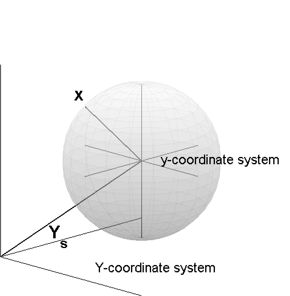
Figure 2: The global ECS \(Y\)-coordinate system and the local \(y\)-coordinate system of the sphere. The sphere is located at position \({\bf Y_s}\). The vector \({\bf x}\) refers to a point on the surface of the sphere..

On a ball¶

We have a ball \(B\) of radius \(\rho\) centered at the origin with a scalar field \(c({\bf y})\) defined in the ball, where \({\bf y}\) is a vector pointing from the origin to a point (\(x,y,z\)) in or on the ball.

The first-order moment-expansion representation of the scalar field \(c({\bf y})\) is

(30)\[\begin{split}\renewcommand{\arraystretch}{1.0} \begin{array}{rcl} c({\bf y}) & = & c^{(0)} + {\bf c^{(1)}} \cdot {\bf y} , %+ \mathcal{O}(\rho^2), \end{array}\end{split}\]

where the coefficients \(c^{(0)} \in \mathbb{R}\) and \({\bf c^{(1)}} \in \mathbb{R}^3\) are given by the moment equations

(31)\[\begin{split}\renewcommand{\arraystretch}{2.0} \begin{array}{rcl} c^{(0)} & = & \frac{3}{4\pi \rho^3} \int_{B} dB\; c({\bf y}) \\ {\bf c^{(1)}} & = & \frac{15}{4\pi \rho^5} \int_{B} dB\; c({\bf y}) \; {\bf y}, \end{array}\end{split}\]

with units \(\left[ c \right]\) and \(\frac{[c]}{L}\), respectively.

Ball gradient¶

(32)\[\begin{split}\renewcommand{\arraystretch}{1.0} \begin{array}{rcl} {\bf \nabla} c ({\bf y}) & \approx & {\bf \nabla} \left( c^{(0)} + {\bf c^{(1)}}\cdot {\bf y} \right) = {\bf \nabla}\left( {\bf c^{(1)}}\cdot {\bf y} \right) , \end{array}\end{split}\]

where \({\bf y} = y_1 \hat{x} + y_2 \hat{y} + y_3 \hat{z}\) is the vector from the origin to the point \((x,y,z)\) in the sphere. Using the vector identity (121) and the fact that \({\bf c^{(1)}}\) is a constant vector,

(33)\[\begin{split}\renewcommand{\arraystretch}{1.0} \begin{array}{rcl} {\bf \nabla} c({\bf y}) & = & \left( {\bf c^{(1)}} \cdot {\bf \nabla} \right) {\bf y} + {\bf c^{(1)}} \times \left( {\bf \nabla} \times {\bf y} \right) \\ & = & \left( {\bf c^{(1)}} \cdot {\bf \nabla} \right) {\bf y} \\ & = & {\bf c^{(1)}} \end{array}\end{split}\]

since \({\bf \nabla} \times {\bf y}=0\) and \(\frac{\partial {\bf y}}{\partial y_i} = \hat{y}_i\).

(34)\[\begin{split}\boxed{ \renewcommand{\arraystretch}{1.0} \begin{array}{rcl} {\bf \nabla} c({\bf y}) & = & {\bf c^{(1)}} \end{array} }\end{split}\]

Ball laplacian¶

The result of application of the laplacian operator to a scalar field defined in the ball \(B\) can be resolved into its moment expansion terms

(35)\[\begin{split}\renewcommand{\arraystretch}{1.0} \begin{array}{rcl} \nabla^2 c({\bf y}) & = & l^{(0)} + {\bf l^{(1)}}\cdot {\bf y} \end{array}\end{split}\]

with units of \(\frac{\#}{L^5}\) and \(\frac{\#}{L^6}\) for the coefficients \(l^{(0)}\) and \({\bf l^{(1)}}\) , respectively.

Zeroth moment. The zeroth moment is given by

(36)\[\begin{split}\renewcommand{\arraystretch}{1.0} \begin{array}{rcl} l^{(0)} & = & \frac{3}{4\pi \rho^3} \int_{B} dB\; \nabla^2 c({\bf y}) \end{array}\end{split}\]

We will use the divergence theorem,

(37)\[\renewcommand{\arraystretch}{1.0} \begin{array}{rcl} \int_{B} dB\; \nabla^2 f({\bf y}) = \int_{S} dS\; \nabla f({\bf x}) \cdot \hat{\bf x} , \end{array}\]

where \(\hat{\bf x}\) is the (outward-pointing) unit normal vector to the surface. Application to (36) gives

(38)\[\renewcommand{\arraystretch}{2.0} \begin{array}{rcl} l^{(0)} = \frac{3}{4\pi \rho^3} \int_{B} dB\; \nabla^2 c({\bf y}) = \frac{3}{4\pi \rho^3 } \int_{S} dS\; \nabla c({\bf x}) \cdot {\bf \hat{x}}. \end{array}\]

Equation (38) shows that the coefficient for the zeroth-moment expansion term is zero in the interior of the ball and specified by the boundary conditions at the surface of the ball.

First moment.

Focusing on the first moment

(39)\[\begin{split}\renewcommand{\arraystretch}{1.0} \begin{array}{rcl} {\bf l^{(1)}} & = & \frac{15}{4\pi \rho^5} \int_{B} dB\; \nabla^2 c({\bf y}) \; {\bf y} . \end{array}\end{split}\]

Applying (126) to (39) gives

(40)\[\begin{split}\renewcommand{\arraystretch}{1.0} \begin{array}{rcl} \frac{15}{4\pi \rho^5} \int_{V} dB\; \left[ \nabla^2 c({\bf y},t) \right] \, {\bf y} & = & \frac{15}{4\pi \rho^4} \int_S dS\; {\bf \hat{x}} {\bf \hat{x}} \cdot {\bf \nabla} c(\rho {\bf \hat{x}} ) - \frac{15}{4\pi \rho^5} \int_B dB\; \nabla c . \end{array}\end{split}\]

Applying (34) to the second term on the right-hand side of the above equation gives

(41)\[\renewcommand{\arraystretch}{1.0} \begin{array}{rcl} -\frac{15}{4\pi \rho^5} \int_B dB\; \nabla c =-\frac{15}{4\pi \rho^5} \frac{4\pi \rho^3 }{3} {\bf c}^{(1)} = -\frac{5}{\rho^2} {\bf c}^{(1)}. \end{array}\]

Gathering the results above, we see that the first-order moment-expansion coefficients resulting from application of the Laplacian to a scalar field in the ball are given by

(42)\[\begin{split}\boxed{ \renewcommand{\arraystretch}{2.0} \begin{array}{rcl} \nabla^2 c({\bf y}) & \approx & l^{(0)} + {\bf l^{(1)} } \cdot {\bf y} \\ l^{(0)} & = & \frac{3}{4\pi \rho^3 } \int_{S} dS\; \nabla c({\bf x}) \cdot {\bf \hat{x}} \\ {\bf l^{(1)}} & = & \frac{15}{4\pi \rho^4} \int_S dS\; {\bf \hat{x}} {\bf \hat{x}} \cdot {\bf \nabla} c(\rho {\bf \hat{x}} ) - \frac{5}{\rho^2} {\bf c}^{(1)} . \end{array} }\end{split}\]

This can seem confusing at first because the surface integral terms, which are only defined on the surface of the ball (\({\bf y}={\bf x}\)), contribute to the scalar field everywhere (all \({\bf y}\)). For instance, in the case of an interpolated scalar field, the flux terms would only contribute to the interpolated nodes at, or in the vicinity of, the surface of the sphere. In the case of moment-expansion fields however, these terms contribute to the calculation of the moments which are used to calculate the value of the field everywhere.

Ball diffusion equation¶

The rate of change of the concentration \(f({\bf y})\) of a molecular species in the ball due to diffusion can be written as a first-order moment-expansion scalar field

(43)\[\frac{\partial f({\bf y})}{\partial t} = \, \zeta\; \nabla^2 f({\bf y}) \approx \, \zeta\; \left( l^{(0)} + {\bf l^{(1)}} \cdot {\bf y} \right),\]

where \(\zeta\) is the diffusion coefficient \(\left(\!\! \mbox{units } \frac{L^2}{T} \right)\) and \(l^{(0)}\) and \({\bf l^{(1)}}\) are defined in (42).

We will utilize Fick’s law,

(44)\[\begin{split}\renewcommand{\arraystretch}{1.0} \begin{array}{rcl} \phi({\bf x}) & = & - \, \zeta\; {\bf \nabla} f({\bf x}) \cdot {\bf \hat{n}}, \end{array}\end{split}\]

where \(\phi({\bf x})\) is the flux through the surface at \({\bf x}\), flux is defined to be the amount of material per unit area per time \(\left([\phi] = \frac{\#}{T L^2}\right)\) moving through a surface, and \({\bf \hat{n}}\) is the outward-pointing normal to the surface.

Then using (42) in the diffusion equation (43) and utilizing (44), the moment-expansion representation of the rate of change of \(f({\bf y})\) due to diffusion is

(45)\[\begin{split}\frac{\partial f({\bf y})}{\partial t} & = & \zeta \left[ \frac{3}{4\pi \rho^3 } \int_{S} dS\; \nabla f({\bf x}) \cdot {\bf \hat{x}} \;\right] + \zeta\; \left[ \frac{15}{4\pi \rho^4} \int_S dS\; {\bf \hat{x}} {\bf \hat{x}} \cdot {\bf \nabla} f(\rho {\bf \hat{x}} ) -\frac{5}{\rho^2} {\bf f}^{(1)} \right] \cdot {\bf y} \\ & = & - \frac{3}{\rho} \frac{1}{4\pi \rho^2} \int_{S} dS\; \phi({\bf x}) \; - \left[ \frac{15}{4\pi \rho^4 } \int_S dS\; \frac{{\bf x} }{\rho} \phi({\bf x}) - \frac{5}{\rho^2} \, \zeta\; {\bf f}^{(1)} \right] \cdot {\bf y}.\end{split}\]

Note that the flux is a scalar field defined on the sphere and can be approximated by a first-order moment-expansion scalar field on the surface of the sphere

(46)\[\begin{split}\phi({\bf x}) & = & \phi^{(0)} + {\bf \phi}^{(1)} \cdot {\bf x} \\ \phi^{(0)} & = & \frac{1}{4\pi \rho^2} \int_{S} dS\; \phi({\bf x}) \\ {\bf \phi^{(1)}} & = & \frac{3}{4\pi \rho^4} \int_{S} dS\; \phi({\bf x}) \; {\bf x} .\end{split}\]

Then the first-order moment-expansion representation of the rate of change of \(c({\bf y})\) (45) becomes

(47)\[\begin{split}\frac{\partial f({\bf y})}{\partial t} & = & - \frac{3}{\rho} \phi^{(0)} - \left[ \frac{5}{\rho} {\bf \phi^{(1)}} + \frac{5}{\rho^2} \, \zeta\; {\bf f}^{(1)} \right] \cdot {\bf y}\end{split}\]

Checking units:

\[\begin{split}[\phi({\bf x})] = [ \phi^{(0)} ] & = & \frac{\#}{TL^2} \hspace{10mm} \left[ {\bf \phi^{(1)} } \right] = \frac{\#}{TL^3} \\ \left[ \frac{\partial f({\bf x})}{\partial t} \right] & = & \frac{\#}{T L^3} \\ \left[ \frac{3}{\rho} \phi^{(0)} \right] & = & \frac{\#}{TL^3} \\ \left[ \frac{5}{\rho} {\bf \phi^{(1)}} \cdot {\bf x} \right] & = & \frac{1}{L} \frac{\#}{T L^3} L \\ \left[ \frac{5}{\rho^2} \zeta {\bf f}^{(1)}\cdot {\bf y} \right] & = & \frac{1}{L^2} \frac{L^2}{T } \frac{\#}{L^4} L = \frac{\#}{T L^3}\end{split}\]

Ball-sphere boundary reactions¶

We have a ball \(B\) of radius \(\rho\) centered at the origin with a two-dimensional concentration of receptor \(r({\bf x},t)\) and complex \(c({\bf x},t)\) on the surface \(S\) of the sphere, where \({\bf x}\) is a vector pointing from the origin to the sphere surface. We have a concentration of ligand \(l({\bf y},t)\) in the three-dimensional space of the interior of the ball \(B\), where \({\bf y}\) is a vector from the origin.

Boundary association: ligand/receptor binding

Ligand binds receptor on the surface of the sphere according to the reaction

(48)\[R + L \xrightarrow{k_1^+} C .\]

Ignoring diffusion, the concentrations evolve according to the relation

(49)\[\begin{split}- \phi_L = - \frac{\partial r}{\partial t}({\bf y},t) = \frac{\partial c}{\partial t}({\bf y},t) & = & {k_1^+}\, l({\bf y(x)},t) \, r({\bf x},t),\end{split}\]

where \(\phi_L\) is the flux of ligand at the surface due to the reaction. The right-hand side of (49) can be represented as a first-order moment expansion on the surface of the sphere

(50)\[{k_1^+}\, l({\bf y(x)},t) \, r({\bf x},t) \approx f^{(0)} + {\bf f^{(1)}} \cdot {\bf y} ,\]

with the following moment-expansion terms

Zeroth moment:

(51)\[\begin{split} \hspace{-10mm} \frac{1}{4\pi \rho^2} \int_{S} dS\;{k_1^+}\, l({\bf y(x)},t) \, r({\bf x}) & \approx & \frac{1}{4\pi \rho^2} \int_{S} dS\;{k_1^+}\, \left( l^{(0)} + {\bf l^{(1)}} \cdot {\bf x} \right) \left( r^{(0)} + {\bf r^{(1)}} \cdot {\bf x} \right) \\ & = & \frac{1}{4\pi \rho^2} \int_{S} dS\;{k_1^+}\, \left( l^{(0)} r^{(0)} + r^{(0)} {\bf l^{(1)}} \cdot {\bf x} + l^{(0)} {\bf r^{(1)}} \cdot {\bf x} + {\bf l^{(1)}} \cdot {\bf x} {\bf r^{(1)}} \cdot {\bf x} \right) \\ & = & {k_1^+}\, l^{(0)} r^{(0)} + \frac{1}{4\pi \rho^2} \int_{S} dS\;{k_1^+}\, \left( r^{(0)} {\bf l^{(1)}} \cdot {\bf x} + l^{(0)} {\bf r^{(1)}} \cdot {\bf x} + {\bf l^{(1)}} \cdot {\bf x} {\bf r^{(1)}} \cdot {\bf x} \right) \\ & = & {k_1^+}\, l^{(0)} r^{(0)} \;\;\;\; \mbox{(to first order)}.\end{split}\]

(52)\[\begin{split} c^{(0)} & = & {k_1^+}\, l^{(0)} r^{(0)}\end{split}\]

First moment:

(53)\[\begin{split} {\bf c^{(1)}} & = & \frac{3}{4\pi \rho^4} \int_{S} dS\; {k_1^+}\, l({\bf y(x)},t) \, r({\bf x}) \cdot {\bf y}\end{split}\]

We will make use of

(54)\[\begin{split} \renewcommand{\arraystretch}{2} \begin{array}{rcl} \int_{S} dS \;\; \left( {\bf a} \cdot {\bf\hat{u}} \right) \hat{\bf u} & = & \frac{4 \pi}{3} \rho^2 {\bf a}. \end{array}\end{split}\]

Then

(55)\[\begin{split} {\bf c^{(1)}} & = & \frac{3}{4\pi \rho^4} \int_{S} dS\; {k_1^+}\, l({\bf y(x)},t) \, r({\bf x}) {\bf x} \\ & = & \frac{3}{4\pi \rho^4} \int_{S} dS\; {k_1^+}\, \left( l^{(0)} + {\bf l^{(1)}} \cdot {\bf x} \right) \left( r^{(0)} + {\bf r^{(1)}} \cdot {\bf x} \right) {\bf x} \\ & = & \frac{3}{4\pi \rho^4} \int_{S} dS\; {k_1^+}\, \left( l^{(0)} r^{(0)} + r^{(0)} {\bf l^{(1)}} \cdot {\bf x} + l^{(0)} {\bf r^{(1)}} \cdot {\bf x} + {\bf l^{(1)}} \cdot {\bf x} {\bf r^{(1)}} \cdot {\bf x} \right) {\bf x} \\ & = & \frac{3}{4\pi \rho^4} \int_{S} dS\; {k_1^+}\, \left( r^{(0)} {\bf l^{(1)}} \cdot {\bf x} + l^{(0)} {\bf r^{(1)}} \cdot {\bf x} + {\bf l^{(1)}} \cdot {\bf x} {\bf r^{(1)}} \cdot {\bf x} \right) {\bf x} \\ & = & \frac{3}{4\pi \rho^4} \int_{S} dS\; {k_1^+}\, \left( r^{(0)} {\bf l^{(1)}} \cdot {\bf x} + l^{(0)} {\bf r^{(1)}} \cdot {\bf x} \right) {\bf x} \;\;\; \mbox{ (to first order) } \\ & = & {k_1^+}\, \left( r^{(0)} {\bf l^{(1)}} + l^{(0)} {\bf r^{(1)}} \right)\end{split}\]

and

(56)\[\begin{split} {\bf c^{(1)}} & = & {k_1^+}\, \left( r^{(0)} {\bf l^{(1)}} + l^{(0)} {\bf r^{(1)}} \right)\end{split}\]

In summary, for the case of a boundary association reaction the ligand flux is given by

(57)\[\begin{split} - \phi_L = - \frac{\partial r}{\partial t}({\bf x},t) = \frac{\partial c}{\partial t}({\bf x},t) & = & {k_1^+}\, l({\bf y(x)},t) \, r({\bf x},t) \\ & \approx & c^{(0)} + {\bf c^{(1)}} \cdot {\bf x} \\ & \approx & {k_1^+}\, l^{(0)} r^{(0)} + {k_1^+}\, \left( r^{(0)} {\bf l^{(1)}} + l^{(0)} {\bf r^{(1)}} \right) \cdot {\bf x} .\end{split}\]

The boundary association dynamics can be written in terms of the dynamics of the moment-expansion coefficients for the flux, receptor, and complex

(58)\[\begin{split} - \phi^{(0)} = - \frac{\partial r^{(0)}}{\partial t}({\bf x},t) = \frac{\partial c^{(0)}}{\partial t}({\bf x},t) & = & {k_1^+}\, l^{(0)} r^{(0)} \\ - {\bf \phi^{(1)}} = -\frac{\partial {\bf r}^{(1)}}{\partial t}({\bf x},t) = \frac{\partial {\bf c}^{(1)}}{\partial t}({\bf x},t) & = & {k_1^+}\, \left( r^{(0)} {\bf l^{(1)}} + l^{(0)} {\bf r^{(1)}} \right) .\end{split}\]

Using (47), the rate of change of the ligand due to the reaction flux is

(59)\[\begin{split} \frac{\partial f({\bf y},t)}{\partial t} & = & - \frac{3}{\rho} \phi^{(0)} - \frac{5}{\rho} {\bf \phi^{(1)}} \cdot {\bf y} \\ & = & \frac{3}{\rho} {k_1^+}\, l^{(0)} r^{(0)} + \frac{5}{\rho} {k_1^+}\, \left( r^{(0)} {\bf l^{(1)}} + l^{(0)} {\bf r^{(1)}} \right) \cdot {\bf y} .\end{split}\]

Boundary dissociation

Complex on the surface of the sphere dissociates according to the reaction

(60)\[\begin{split}C & \xrightarrow{k_1^-} & R + L .\end{split}\]

Ignoring diffusion, the concentrations evolve according to the relation

(61)\[\begin{split} \phi_L = \frac{\partial r}{\partial t}({\bf x},t) = - \frac{\partial c}{\partial t}({\bf x},t) & = & {k_1^{-}} c({\bf x},t).\end{split}\]

where \(\phi_L\) is the flux of ligand at the surface due to the reaction. The right-hand side of (61) can be represented as a first-order moment expansion

(62)\[ {k_1^{-}} c({\bf x},t) \approx f^{(0)} + {\bf f^{(1)}} \cdot {\bf x} ,\]

with the following moment-expansion terms

Zeroth moment:

(63)\[\begin{split} f^{(0)} & = & \frac{1}{4\pi \rho^2} \int_{S} dS\; {k_1^{-}} c({\bf x}) \\\end{split}\]

(64)\[\begin{split} \frac{1}{4\pi \rho^2} \int_{S} dS\; {k_1^{-}} c({\bf x},t) & \approx & \frac{1}{4\pi \rho^2} \int_{S} dS\; {k_1^{-}} \left( c^{(0)} + {\bf c^{(1)}} \cdot {\bf x} \right) = {k_1^{-}} c^{(0)}\end{split}\]

(65)\[\begin{split} f^{(0)} & = & {k_1^{-}} c^{(0)}\end{split}\]

First moment

(66)\[\begin{split} {\bf f^{(1)}} & = & \frac{3}{4\pi \rho^4} \int_{S} dS\; {k_1^{-}} c({\bf x}) \cdot {\bf y}\end{split}\]

We will make use of

(67)\[\begin{split} \int_{S} dS \;\; \left( {\bf a} \cdot {\bf\hat{u}} \right) \hat{\bf u} & = & \frac{4 \pi}{3} \rho^2 {\bf a}\end{split}\]

Then

(68)\[\begin{split} {\bf f^{(1)}} & = & \frac{3}{4\pi \rho^4} \int_{S} dS\; {k_1^{-}} c({\bf x}) {\bf x} = \frac{3}{4\pi \rho^4} \int_{S} dS\; {k_1^{-}} \left( c^{(0)} + {\bf c^{(1)}} \cdot {\bf x} \right) {\bf x} = \frac{3}{4\pi \rho^4} \int_{S} dS\; {k_1^{-}} {\bf c^{(1)}} \cdot {\bf x} \; {\bf x} \\ & = & {k_1^{-}} {\bf c^{(1)}}\end{split}\]

(69)\[\begin{split} {\bf f^{(1)}} & = & {k_1^{-}} {\bf c^{(1)}}\end{split}\]

In summary, for the case of a boundary dissociation reaction

(70)\[\begin{split} \phi_L = \frac{\partial r}{\partial t}({\bf x},t) = - \frac{\partial c}{\partial t}({\bf x},t) & = & {k_1^{-}} c({\bf x},t) = {k_1^{-}} \left( c^{(0)} + {\bf c^{(1)}} \cdot {\bf x} \right).\end{split}\]

The boundary dissociation dynamics can be written in terms of the dynamics of the moment-expansion coefficients for the flux, receptor, and complex

(71)\[\begin{split} \phi^{(0)} = \frac{\partial r^{(0)}}{\partial t}({\bf x},t) = - \frac{\partial c^{(0)}}{\partial t}({\bf x},t) & = & {k_1^{-}} c^{(0)} \\ {\bf \phi^{(1)}} = -\frac{\partial {\bf r}^{(1)}}{\partial t}({\bf x},t) = \frac{\partial {\bf c}^{(1)}}{\partial t}({\bf x},t) & = & {k_1^{-}}\, {\bf c^{(1)}}\end{split}\]

Using (47), the rate of change of the ligand due to the dissociation reaction flux is

(72)\[\begin{split} \frac{\partial f({\bf y},t)}{\partial t} & = & - \frac{3}{\rho} \phi^{(0)} - \frac{5}{\rho} {\bf \phi^{(1)}} \cdot {\bf y} \\ & = & - {k_1^{-}} \left( \frac{3}{\rho} c^{(0)} + \frac{5}{\rho} {\bf c^{(1)}} \cdot {\bf y} \right)\end{split}\]

Catalyzed boundary activation

Molecule \(A\) inside the sphere binds to complex \(C\) on the surface of the sphere. Activated (driver) molecule \(A^{*}\) deactivates to \(A\).

(73)\[\begin{split}\renewcommand{\arraystretch}{1.0} \begin{array}{rcl} A + C & \xrightarrow{k_1} & C + A{^*}\\ A^{*} & \xrightarrow{k_2} & A \end{array}\end{split}\]

The dynamical equation governing the activated driver concentration is (neglecting diffusion)

(74)\[\begin{split} \phi_{a*} & = & k_1 a({\bf y(x)},t) \, c({\bf x},t) - k_2 a^{*}({\bf y(x)},t) \approx f^{(0)} + {\bf f^{(1)} } \cdot {\bf y},\end{split}\]

where in the last equation on the right-hand side we are representing the time rate of change of \(a^{*} ({\bf y},t)\) as a first-order moment expansion with coefficients

Zeroth moment:

First term on the right-hand side

(75)\[\begin{split}\begin{array} f_1^{(0)} & = & \frac{3}{4\pi \rho^3} \int_{B} dB\; k_1 a({\bf y(x)},t) \, c({\bf x},t) \\ & \approx & \frac{3}{4\pi \rho^3} \int_{S} dS\; k_1 \left[ \left(a^{(0)} + {\bf a^{(1)} } \cdot {\bf x}\right) + \left(c^{(0)} + {\bf c^{(1)} } \cdot {\bf x}\right) \right] = \frac{3}{\rho} k_1 a^{(0)} c^{(0)} \end{array}\end{split}\]

Second term on the right-hand side

(76)\[\begin{split} f_2^{(0)} & = & - \frac{3}{4\pi \rho^3} \int_{B} dB\; k_2 a^{*}({\bf y(x)},t) = - k_2 a^{*(0)}\end{split}\]

First moment:

First term on the right-hand side

(77)\[\begin{split} {\bf f_1^{(1)}} & = & \frac{15}{4\pi \rho^5} \int_{B} dB\; \; k_1 a({\bf y(x)},t) \, c({\bf x},t) \cdot {\bf y} \\ & \approx & k_1 \frac{15}{4\pi \rho^5} \int_{S} dS\; \left[ \left(a^{(0)} + {\bf a^{(1)} } \cdot {\bf x}\right) + \left(c^{(0)} + {\bf c^{(1)} } \cdot {\bf x}\right) \right] \cdot {\bf x} \\ & = & \frac{5}{\rho} k_1 \left( a^{(0)} {\bf c^{(1)}} + c^{(0)} {\bf a^{(1)}} \right) \;\; \mbox{(to first order)}\end{split}\]

Second term on the right-hand side

(78)\[\begin{split} {\bf f_2^{(1)}} & = & - \frac{15}{4\pi \rho^5} \int_{B} dB\; \; k_2 a^{*}({\bf y(x)},t) \cdot {\bf y} = - k_2 {\bf a^{*(1)}}\end{split}\]

Summary:

(79)\[ \phi_{a*} = \left( \frac{3}{\rho} k_1 a^{(0)} c^{(0)} - k_2 a^{*(0)} \right) + \left[ \frac{5}{\rho} k_1 \left( a^{(0)} {\bf c^{(1)}} + c^{(0)} {\bf a^{(1)}} \right) - k_2 {\bf a^{*(1)}} \right] \cdot {\bf x}\]

Discretized scalar fields¶

A time-dependent scalar field \(c({\bf x, t})\) with \({\bf x}\in \mathbb{R}^d\), \(t \in (0, \infty)\) in \(d\)-dimensional space, can be approximated by a discretized scalar field of the form

(80)\[\begin{split} c({\bf x}) & \approx & \sum_{i=1}^{N} c_{i}(t) \psi_i({\bf x}),\end{split}\]

where \(C_{i}\) is the value of the scalar field at the \(i\) th point, \(N = \prod_{i=1}^{d} n_i\), \(\,n_i\) is the number of lattice points in the \(i\) th dimension, \(d\) is the dimension of the space, and \(\psi_i\) are interpolation functions. We assume that the node points are uniformly spaced with grid-step \(h\) the same in all dimensions, and use the notation \({\bf x^{(n)}}=(x_{1}^{(n)},x_{2}^{(n)},\ldots, x_{d}^{(n)})\) to designate the \(n\) th lattice point.

Three-dimensional space: derivatives at lattice points¶

We will make use of the Taylor expansion for functions with three-dimensional spatial dependence

(81)\[\begin{split} f( {\bf x} + {\bf h} ) & \approx & f( {\bf x} ) + \sum_{i=1}^3 \frac{ \partial f({\bf x})}{\partial x_i} h + \frac{1}{2!} \sum_{i=1}^3 \sum_{j=1}^3 \frac{ \partial^2 f({\bf x}) }{\partial x_i \partial x_j} h^2 + \mathcal{O}(h^3).\end{split}\]

We will also make use of the notation \({\bf h}_i \equiv ( \delta_{i1}, \delta_{i2}, \delta_{i3})h\), where \(\delta_{ij}\) is the Kronecker delta

(82)\[\begin{split} \delta_{ij} & = & \left\{ \begin{array}{rr} 0 & i \ne j \\ 1 & i = j \end{array} \right. .\end{split}\]

Gradient¶

To approximate first derivative in the \(x_1\)-direction at the lattice points, we use \({\bf h}=(\pm h,0,0)\) with the Taylor expansions (81). Then

(83)\[\begin{split} f({\bf x}^{(n)} + {\bf h}) & \approx & f({\bf x}^{(n)}) +\frac{\partial f({\bf x}^{(n)})}{\partial x_1} h + \frac{1}{2!} \frac{\partial^2 f({\bf x}^{(n)})}{\partial x_1^2 } h^2 + \mathcal{O}(h_1^3) \\ f({\bf x}^{(n)} - {\bf h}) & \approx & f({\bf x}^{(n)}) - \frac{\partial f({\bf x}^{(n)})}{\partial x_1} h + \frac{1}{2!} \frac{\partial^2 f({\bf x}^{(n)})}{\partial x_1^2 } h^2 + \mathcal{O}(h_1^3) .\end{split}\]

Subtracting the two equations above gives the \(x_1\)-derivative to first order at the \(n\text{th}\) lattice point

(84)\[\begin{split} \frac{\partial f({\bf x}^{(n)})}{\partial x_1} & \approx & \frac{ f({\bf x}^{(n)}+h) - f({\bf x}^{(n)}-h_1) }{2 h} + \mathcal{O}(h^2) .\end{split}\]

Generalizing to other dimensions and using (84) and (82), the gradient operator to first order (in a rectilinear coordinate-system) is

(85)\[ \nabla f({\bf x}^{(n)}) = \sum_{i=1}^3 \frac{\partial f({\bf x}^{(n)})}{\partial x_i} {\bf\hat{x}_i} \approx \sum_{i=1}^3 \frac{1}{2 h} \left[ f( {\bf x}^{(n)} + {\bf h}_i ) - f( {\bf x}^{(n)} - {\bf h}_i ) \right] {\bf\hat{x}_i},\]

where \({\bf\hat{x}_i}\) is the unit vector in the \(i\text{th}\) dimension.

Gradient at boundary nodes¶

We only consider boundary surfaces whose unit normal are coincident with the rectilinear axes of the space.

The central differences in (85) cannot be evaluated at the boundaries. To approximate the gradient at the boundary, we use a polynomial approximation of the function to get a first order estimate of the derivative in the direction perpendicular to the boundary surface. For example, in the vicinity of the boundary point \((x_1=0, x_2, x_3)\), we approximate the function as \(f(x_1,x_2,x_3) \approx c_0 + c_1 x_1 + c_2 x_1^2\). Then,

(86)\[\begin{split} \renewcommand{\arraystretch}{2} \begin{array}{rcl} f(0,x_2,x_3) & \approx & c_0 \\ f(h,x_2,x_3) & \approx & c_0 + c_1 h + c_2 h^2 \\ f(2h,x_2,x_3) & \approx & c_0 +2 c_1 h + 4 c_2 h^2 \end{array}\end{split}\]

Solving for the coefficients \(c_0\) and \(c_1\) gives

(87)\[\begin{split} \renewcommand{\arraystretch}{2} \begin{array}{rcl} c_0 & = & f(0,x_2,x_3) \\ c_1 & = & (2h)^{-1} \left[ - 3f(0,x_2,x_3)+ 4f(h,x_2,x_3) - f(2h,x_2,x_3) \right] \end{array}\end{split}\]

Differentiating the polynomial and evaluating at \(x=0\) gives

(88)\[ \left. \frac{df(x_1,x_2,x_3)}{dx_1} \right|_{(0,x_2,x_3)} = c_1 = (2h)^{-1} \left[ - 3f(0)+ 4f(h,x_2,x_3) - f(2h,x_2,x_3) \right],\]

which approximates the derivative in the direction perpendicular to the boundary in terms of the values at the boundary node and neighbor nodes.

Similarly, in the vicinity of the boundary point \((x_1=L, x_2, x_3)\) we approximate the function as \(f(x_1,x_2,x_3) \approx c_0 + c_1 x_1 + c_2 x_1^2\). Then,

(89)\[\begin{split} \renewcommand{\arraystretch}{2} \begin{array}{rcl} f(L,x_2,x_3) & \approx & c_0 + c_1 L + c_2 L^2 \\ f(L-h,x_2,x_3) & \approx & c_0 + c_1 (L-h) + c_2 (L-h)^2 \\ f(L-2h,x_2,x_3) & \approx & c_0 + c_1 (L-2h) + c_2 (L-2h)^2 \end{array}\end{split}\]

From the first equation we obtain \(c_0 = f(L,x_2,x_3) - c_1 L - c_2 L^2\). Multiplying the second equation by 4, subtracting the third equation and using the above result, gives

(90)\[\begin{split} c_1 + 2 L c_2 & = & (2h)^{-1} \left[ 3 f(L,x_2,x_3) - 4 f(L-h,x_2,x_3) + f(L-2h,x_2,x_3) \right]\end{split}\]

Differentiating the polynomial at \(x=L\) and using the result above gives

(91)\[ \left. \frac{df(x_1,x_2,x_3)}{dx_1} \right|_{(L,x_2,x_3)} = c_1 + 2Lc_2 = (2h)^{-1} \left[ 3 f(L,x_2,x_3) - 4 f(L-h,x_2,x_3) + f(L-2h,x_2,x_3) \right].\]

Approximation of the derivatives at other boundaries follow in a similar manner.

Laplacian¶

To approximate second derivatives, we add the two equations in (83). This gives the second derivative in the \(x_1\)-direction (to first order)

(92)\[\begin{split} \frac{ \partial f^2( {\bf x}^{(n)} )}{\partial x_1^2} & \approx & \frac{1}{ h^2} \left( f( {\bf x}^{(n)} + {\bf h_1} ) + f( {\bf x}^{(n)} - {\bf h_1} ) - 2f( {\bf x}^{(n)} ) \right) + \mathcal{O}(h^2)\end{split}\]

where again we are using the notation \({\bf h}_i \equiv ( \delta_{i1}, \delta_{i2}, \delta_{i3})h\).

Generalizing to other dimensions and using (84) and (82), the Laplacian operator to first order (in a rectilinear coordinate-system) is

(93)\[ \nabla^2 f( {\bf x}^{(n)} ) = \sum_{i=1}^3 \frac{\partial^2 f( {\bf x}^{(n)} )}{\partial x_i^2} \approx \sum_{i=1}^3 \frac{1}{h_i^2} \left[ f( {\bf x}^{(n)} + {\bf h}_i ) + f( {\bf x}^{(n)} - {\bf h}_i ) - 2f( {\bf x}^{(n)} )\right] .\]

Diffusion¶

Consider a scalar field \(f({\bf x},t)\) describing the time-dependent concentration of molecules in volume \(V\) with surface \(S\). The time evolution of \(f({\bf x},t)\) due to diffusion is given by

(94)\[\begin{split} \frac{\partial f({\bf x},t)}{\partial t} & = & \zeta \nabla^2 f({\bf x},t),\end{split}\]

subject to boundary conditions

(95)\[ {\bf \nabla} f({\bf x}_s) \cdot {\bf \hat{n}} = - \zeta^{-1}\; \phi({\bf x}_s) \;\; \mbox{ and/or } \;\; f({\bf x}_s) = \mbox{constant}\]

where \(\zeta\) is the diffusion coefficient, \(\phi({\bf x})\) is the flux (amount of material per unit area per time) through a surface element at position \({\bf x}_s\) on \(S\), and \({\bf \hat{n}}\) is the unit normal to the surface, which points out of the volume.

Using (93), the Laplacian applied to lattice points on the interior is, to first order, given by

(96)\[\begin{split} \frac{\partial f({\bf x^{(n)}},t)}{\partial t} & \approx & \zeta \sum_{i=1}^3 \frac{1}{h_i^2} \left[ f( {\bf x^{(n)}} + {\bf h}_i ) + f( {\bf x^{(n)}} - {\bf h}_i ) - 2f({\bf x^{(n)}})\right] ,\end{split}\]

where again \({\bf h}_i \equiv ( \delta_{i1}, \delta_{i2}, \delta_{i3}) h\) and \(\delta_{ij}\) is the Kronecker delta.

Boundary conditions¶

Flux (Neumann)¶

When we impose flux boundary conditions, we specify the flux \({\bf \phi}({\bf x}_s)\) at the surface point \({\bf x}_s\). Then from (96), this imposes a gradient at the surface

(97)\[ \nabla f({\bf x}_s,t) \cdot {\bf \hat{n}} = \sum_{i=1}^{3} \frac{d f({\bf x}_s, t) }{d x_i} n_i = - \frac{\phi({\bf x}_s)}{\zeta} .\]

Flux at natural boundaries

In general, the discretized points of the volume may not be coincident with the discretized points of the surface. Such cases will occur for curved surfaces or for surfaces moving with respect to the volume, such as with cells. We define natural boundaries to be those boundaries for which the lattice points of the surface are coincident with lattice points of the volume.

Consider a lattice point \({\bf x_s}^{(n)}\) on the surface of a volume. Using (96) and (85), the flux condition on the gradient at \({\bf x_s}^{(n)}\) can be written as

(98)\[ \nabla f({\bf x_s}^{(n)},t) \cdot {\bf \hat{n}} = \sum_{i=1}^3 \frac{ n_i}{2 h_i} \left[ f( {\bf x_s}^{(n)} + {\bf h}_i , t) - f( {\bf x_s}^{(n)} - {\bf h}_i, t ) \right] = - \frac{\phi({\bf x_s}^{(n)})}{\zeta} ,\]

where again \({\bf h}_i \equiv ( \delta_{i1}, \delta_{i2}, \delta_{i3}) h\). For \({\bf x_s}^{(n)}\) on the surface, 1 to 3 of the evaluation points \({\bf x}_s^{(n)} \pm {\bf h}_i\) lie outside the volume. We impose the flux by calculating the value of the field at these {it virtual (image)} lattice points as function of the applied flux (using (98)), then substitute these resulting expressions for the virtual points in the application of the Laplacian at the surface point (93).

Let us illustrate with some simple cases.

Consider the scalar field \(f({\bf x}, t)\) defined in the volume \(V\), which is a rectangular prism with extents \(0 \le x_1 \le L_1\), \(0 \le x_2 \le L_2\), and \(0 \le x_3 \le L_3\), with flux \(\phi\) specified at the natural boundaries.

Example 1: Consider the point \(x_1=L_1\) on the boundary , with \({\bf x_{1L}} \equiv (L_1,x_2,x_3)\) and \({\bf \hat{n}} = (1, 0,0)\). Then using (98), we can compute the value of the virtual lattice point \(f(L_1+h_1,x_2,x_3)\)

(99)\[\begin{split} \frac{ 1}{2 h_1} \left[ f(L_1+h_1,x_2,x_3) - f(L_1-h_1,x_2,x_3) \right] & = & - \frac{\phi( L_1,x_2,x_3 )}{\zeta} \\ f(L_1+h_1,x_2,x_3) & = & - \frac{2 h_1 \phi( L_1,x_2,x_3 ) }{\zeta} + f(L_1-h_1,x_2,x_3) .\end{split}\]

Substituting this in the equation for the Laplacian (93) gives the second derivative in the \(x_1\) direction at the boundary point as a function of the applied flux

(100)\[\begin{split} \frac{ \partial f^2( {\bf x_{1L} } )}{\partial x_1^2} & = & \frac{1 }{h_1^2} \left[ f(L_1+h_1,x_2,x_3) + f(L_1-h_1,x_2,x_3) - 2 f(L_1,x_2,x_3) \right] \\ & = & \frac{1}{h_1^2} \left[ - \frac{2 h_1 \phi(L_1,x_2,x_3 ) }{\zeta} + 2 f(L_1-h_1,x_2,x_3) - 2 f(L_1,x_2,x_3) \right] \\ & = & \frac{2}{h_1^2} \left[ f(L_1-h_1,x_2,x_3) - f(L_1,x_2,x_3) \right] - \frac{2 \phi(L_1,x_2,x_3) }{h_1 \zeta} .\end{split}\]

Example 2: Consider the point on the boundary \(x_1=0\), with \({\bf x_{10}} \equiv (0,x_2,x_3)\) and \({\bf \hat{n}} = (-1, 0,0)\). Using (98), we can compute the value of the virtual lattice point \(f(-h_1,x_2,x_3)\)

(101)\[\begin{split} - \frac{ 1}{2 h_1} \left[ f(h_1,x_2,x_3) - f(-h_1,x_2,x_3) \right] & = & - \frac{\phi( 0,x_2,x_3 )}{\zeta} \\ f(-h_1,x_2,x_3) & = & - \frac{2 h_1 \phi(0,x_2,x_3) }{\zeta} + f(h_1,x_2,x_3) .\end{split}\]

Substituting this in the equation for the Laplacian (93) gives the second derivative in the \(x_1\) direction at the boundary point as a function of the applied flux

(102)\[\begin{split} \frac{ \partial f^2( {\bf x_{10} } )}{\partial x_1^2} & = & \frac{1 }{h_1^2} \left[ f(h_1,x_2,x_3) + f(-h_1,x_2,x_3) - 2 f(0,x_2,x_3) \right] \\ & = & \frac{1}{h_1^2} \left[ - \frac{2 h_1 \phi(0,x_2,x_3 ) }{\zeta} + 2 f(h_1,x_2,x_3) - 2 f(0,x_2,x_3) \right] \\ & = & \frac{2}{h_1^2} \left[ f(h_1,x_2,x_3) - f(0,x_2,x_3) \right] - \frac{2 \phi(0,x_2,x_3) }{h_1 \zeta} .\end{split}\]

Flux from a tiny sphere¶

Consider a spherical surface \(S\) with flux \(\phi\) at an arbitrary location \({\bf x_s}\) in the volume \(V\). (In this case, the surface is not a natural boundary.) If the radius \(\rho\) of the sphere is much less than the distance \(h\) between lattice points \(\rho \ll h\), then the flux acts like a point source and the rate of change of the concentration at \({\bf x}_s\) is give by

(103)\[ \frac{ \partial f({\bf x_s})}{\partial t} = \frac{4\pi\rho^2}{h^3} \phi .\]

We use interpolation to distribute the change in concentration to the lattice points of the voxel that contains the point:math:{bf x}_s.

Dirichlet (fixed)¶

A Dirichlet boundary conditions specifies a fixed value \(\psi({\bf x}_s)\) for the function at the boundary point \({\bf x}_s\). Therefore, the value of the function at the boundary does not change in time and

(104)\[ \frac{\partial f({\bf x}_s,t)}{\partial t} = \zeta \nabla^2 f({\bf x}_s,t) = 0 .\]

Toroidal¶

Essentially, there are no boundaries for the toroidal case; material that diffuses through one face enters through the opposite face.

Example 1: Consider the point \(x_1=L_1\) on the boundary, with \({\bf x_{1L}} \equiv (L_1,x_2,x_3)\). Applying the toroidal boundary condition \(f(0,x_2,x_3) = f(L_1,x_2,x_3)\) to the second derivative in the \(x_1\)-direction (92) gives

(105)\[\begin{split} \frac{ \partial f^2( {\bf x_{1L} } )}{\partial x_1^2} & = & \frac{1 }{h_1^2} \left[ f(L_1+h_1,x_2,x_3) + f(L_1-h_1,x_2,x_3) - 2 f(L_1,x_2,x_3) \right] \\ & = & \frac{1 }{h_1^2} \left[ f(h_1,x_2,x_3) + f(L_1-h_1,x_2,x_3) - 2 f(L_1,x_2,x_3) \right]\end{split}\]

Example 2: Consider the point \(x_1=0\) on the boundary, with \({\bf x_{10}} \equiv (0,x_2,x_3)\). Applying the toroidal boundary condition \(f(0,x_2,x_3) = f(L_1,x_2,x_3)\) to the second derivative in the \(x_1\)-direction (92) gives

(106)\[\begin{split} \frac{ \partial f^2( {\bf x_{10} } )}{\partial x_1^2} & = & \frac{1 }{h_1^2} \left[ f(h_1,x_2,x_3) + f(-h_1,x_2,x_3) - 2 f(0,x_2,x_3) \right] \\ & = & \frac{1 }{h_1^2} \left[ f(h_1,x_2,x_3) + f(L_1-h_1,x_2,x_3) - 2 f(0,x_2,x_3) \right]\end{split}\]

Bilinear interpolation¶

We will use the following notation in this section.

grid-spacing \(h\)
\(f^n \equiv f({\bf x^{(n)}})\) is the value of the function at the \(n\text{th}\) node.
\(f^n_x\) (\(f^n_y\)) is the value of the \(x\)-derivative (\(y\)-derivative )at node \(n\) (point \({\bf x^{(n)}}\)).

Figure 3: Node designations for interpolation.

Scalar field interpolation¶

Point \(f^0\) lies in the pixel with surrounding nodes: \(f^1\), \(f^2\), \(f^3\), and \(f^4\) (Figure 3). We use a 2D Taylor expansions about point \(f^0\) to approximate the function at the surrounding nodes

(107)\[\begin{split} f^1 & = & f^0 - \delta_x f^0_x - \delta_y f^0_y + \mathcal{O}(h^2) \\ f^2 & = & f^0 - \delta_x f^0_x + (h - \delta_y) f^0_y + \mathcal{O}(h^2) \\ f^3 & = & f^0 + (h - \delta_x) f^0_x - \delta_y f^0_y + \mathcal{O}(h^2) \\ f^4 & = & f^0 + (h - \delta_x) f^0_x + (h - \delta_y) f^0_y + \mathcal{O}(h^2) .\end{split}\]

Combining the first two and last two equations in (107) gives

(108)\[\begin{split} (h-\delta_y) f^1 + \delta_y f^2 & = & h f^0 - h \delta_x f^0_x + \mathcal{O}(h^3) \\ (h-\delta_y) f^3 + \delta_y f^4 & = & h f^0 + h (h - \delta_x) f^0_x + \mathcal{O}(h^3)\end{split}\]

Combining the equations in (108) gives

(109)\[\begin{split} (h-\delta_x) \left[ (h-\delta_y) f^1 + \delta_y f^2 \right] + \delta_x \left[ (h-\delta_y) f^3 + \delta_y f^4 \right] & = & h^2 f^0 + \mathcal{O}(h^4) .\end{split}\]

Finally,

(110)\[\begin{split} f^0 & \approx & (1-\Delta_x)(1-\Delta_y) f^1 + (1-\Delta_x) \Delta_y f^2 + \Delta_x (1-\Delta_y) f^3 + \Delta_x \Delta_y f^4 + \mathcal{O}(h^2) ,\end{split}\]

where \(\Delta \equiv \frac{\delta}{h}\).

Equation (110) can be easily generalized to the 3D case.

Gradient interpolation¶

Applying the bilinear interpolation equation (110) to the \(x\)-derivative \(f_x^0\) at point \(x^0\) gives

(111)\[\begin{split} f_x^0 & = & (1-\Delta_x)(1-\Delta_y) f_x^1 + (1-\Delta_x) \Delta_y f_x^2 + \Delta_x (1-\Delta_y) f_x^3 + \Delta_x \Delta_y f_x^4 + \mathcal{O}(h^2) .\end{split}\]

Using the first-order approximations for the derivatives at the node points (84)

(112)\[\begin{split} f^1_x & \approx & \frac{1}{2h} \left( f^{3} - f^{9} \right)\\ & \vdots &\end{split}\]

in (111) gives

(113)\[\begin{split} f_x^0 & = & \frac{1}{2h} \left[ (1-\Delta_x)(1-\Delta_y) \left( f^{3} - f^{9} \right) + (1-\Delta_x) \Delta_y \left( f^{4} - f^{10} \right) \right. \\ & & \; \; \; \left. + \; \Delta_x (1-\Delta_y) \left( f^{11} - f^{1} \right) + \Delta_x \Delta_y \left( f^{12} - f^{2} \right) \right] .\end{split}\]

The derivatives calculated with (113) are continuous across nodes.

Base node \((i,j)\).

(114)\[\begin{split} f_x^0 & = & \frac{1}{2h} \left[ (1-\Delta_x)(1-\Delta_y) \left( f(i+1,j) - f(i-1,j) \right) \right. \\ & & \; \; \; \left. \right] .\end{split}\]

Equation (113) can easily be generalized to derivatives in other dimensions and to the 3D case.

Gradient interpolation at boundaries¶

_images/pixel_grad_interpolation_boundary.png

Figure 4: Node designations for interpolation.

Case 1: Consider the case of gradient interpolation at point \(f^0\), which lies in the pixel with surrounding nodes 1,2, 3, an 4, with associated function values \(f^1\), \(f^2\), \(f^3\), and \(f^4\) (Figure 4 (a)), where nodes 1 and 2 lie on the boundary.

Applying the bilinear interpolation equation (110) to the \(x\)-derivative \(f_x^0\) at point \(x^0\) gives

(115)\[\begin{split} f_x^0 & \approx & (1-\Delta_x)(1-\Delta_y) f_x^1 + (1-\Delta_x) \Delta_y f_x^2 + \Delta_x (1-\Delta_y) f_x^3 + \Delta_x \Delta_y f_x^4 .\end{split}\]

Using the first-order approximations for the derivatives at the node points (84) and (91)

(116)\[\begin{split} f^1_x & \approx & \frac{1}{2h} \left[ - 3 f^{1} + 4 f^{3} - f^{11} \right] \\ f^2_x & \approx & \frac{1}{2h} \left[ - 3 f^{2} + 4 f^{4} - f^{12} \right] \\ f^3_x & \approx & \frac{1}{2h} \left( f^{11} - f^{1} \right) \\ f^4_x & \approx & \frac{1}{2h} \left( f^{12} - f^{2} \right) \\\end{split}\]

in (115) gives

(117)\[\begin{split} f_x^0 & \approx & (1-\Delta_x)(1-\Delta_y) \frac{1}{2h} \left[ - 3 f^{1} + 4 f^{3} - f^{11} \right] + (1-\Delta_x) \Delta_y \frac{1}{2h} \left[ - 3 f^{2} + 4 f^{4} - f^{12} \right] \\ & & + \Delta_x (1-\Delta_y) \frac{1}{2h} \left( f^{11} - f^{1} \right) + \Delta_x \Delta_y \frac{1}{2h} \left( f^{12} - f^{2} \right) .\end{split}\]

Case 2: Consider the case of gradient interpolation at point \(f^0\), which lies in the pixel with surrounding nodes 1,2, 3, an 4, with associated function values \(f^1\), \(f^2\), \(f^3\), and \(f^4\) (Figure 4 (b)), where nodes 3 and 4 lie on the boundary.

Applying the bilinear interpolation equation (110) to the \(x\)-derivative \(f_x^0\) at point \(x^0\) gives

(118)\[\begin{split} f_x^0 & \approx & (1-\Delta_x)(1-\Delta_y) f_x^1 + (1-\Delta_x) \Delta_y f_x^2 + \Delta_x (1-\Delta_y) f_x^3 + \Delta_x \Delta_y f_x^4 .\end{split}\]

Using the first-order approximations for the derivatives at the node points (84) and (91)

(119)\[\begin{split} f^1_x & \approx & \frac{1}{2h} \left( f^{3} - f^{9} \right) \\ f^2_x & \approx & \frac{1}{2h} \left( f^{4} - f^{10} \right) \\ f^3_x & \approx & \frac{1}{2h} \left[ 3 f^{3} - 4 f^{1} + f^{9} \right] \\ f^4_x & \approx & \frac{1}{2h} \left[ 3 f^{4} - 4 f^{2} + f^{10} \right]\end{split}\]

in (118) gives

(120)\[\begin{split} f_x^0 & \approx & (1-\Delta_x)(1-\Delta_y) \frac{1}{2h} \left( f^{3} - f^{9} \right) + (1-\Delta_x) \Delta_y \frac{1}{2h} \left( f^{4} - f^{10} \right) \\ & & + \Delta_x (1-\Delta_y) \frac{1}{2h} \left[ 3 f^{3} - 4 f^{1} + f^{9} \right] + \Delta_x \Delta_y \frac{1}{2h} \left[ 3 f^{4} - 4 f^{2} + f^{10} \right] .\end{split}\]

Helpful identities¶

This is a collection of identities, proofs, etc. to aid the presentation in the previous sections.

Standard vector identities¶

(121)\[ \renewcommand{\arraystretch}{2} \begin{array}{rcl} {\bf \nabla} \left( {\bf a}\cdot {\bf b} \right) = \left( {\bf a}\cdot {\bf \nabla} \right) {\bf b} + \left( {\bf b}\cdot {\bf \nabla} \right) {\bf a} + {\bf a} \times \left( {\bf \nabla} \times {\bf b} \right) + {\bf b} \times \left( {\bf \nabla} \times {\bf a} \right) \end{array}\]

Vector identities¶

Identity 1¶

For a scalar field \(a({\bf y})\) with \({\bf y} = y_1{\bf\hat{x}_1} + y_2{\bf\hat{x}_2} + z{\bf\hat{x}_3}\) a vector from the origin to point \((y_1,y_2,y_3)\), if \(F \equiv \left( \nabla^2 a({\bf y}) \right) {\bf y}\) then if follows that :math:` F = left( sum_i partial_i^2 a({bf y}) right) {bf y}mbox{ }` and

(122)\[\begin{split} \renewcommand{\arraystretch}{1} \begin{array}{rcl} F_j & = & \sum_i \partial_i^2 a({\bf y}) \; y_j \\ F_j & = & \sum_i \partial_i \left(\partial_i a({\bf y}) \; y_j \right) - \sum_i \partial_i a({\bf y}) \; \partial_i y_j \\ F_j & = & \sum_i \partial_i \left(\partial_i a({\bf y}) \; x_j \right) - \partial_j a({\bf x}) y_j, \end{array}\end{split}\]

since \(\partial_i y_j=\delta_{ij} y_j\).

But

(123)\[\begin{split} \renewcommand{\arraystretch}{1} \begin{array}{rcl} F_j & = & \sum_i \partial_i \left(\partial_i a({\bf x}) \; y_j \right) - \partial_j a({\bf y}) y_j = \sum_i \partial_i \left(y_j \; \partial_i a({\bf y}) \right) - \partial_j a({\bf y}) y_j \end{array}\end{split}\]

Then

(124)\[ \boxed{ \renewcommand{\arraystretch}{1} \begin{array}{rcl} \sum_i \partial_i \left(\partial_i a({\bf y})\; {\bf y} \right) = \sum_i \partial_i \left(({\bf y} \; \partial_i a({\bf y}) \right) = \left( \nabla^2 a({\bf y}) \right) {\bf y} + \nabla a \; {\bf y} \end{array} }\]

Divergence theorem,

(125)\[\begin{split} \renewcommand{\arraystretch}{1} \begin{array}{rcl} \int_V dV\, \left( {\bf \nabla} \cdot {\bf A} \right) & = & \int_S dS\, {\bf A} \cdot {\bf \hat{n}}, \end{array}\end{split}\]

where \({\bf A}\) is a vector and \({\bf \hat{n}}\) is the normal to the surface.

Identity 2¶

Ball \(B\) of radius \(\rho\) centered at the origin, Scalar field \(a( {\bf y} )\) with \({\bf y} = y_1{\bf\hat{x}_1} + y_2{\bf\hat{x}_2} + z{\bf\hat{x}_3}\) a vector from the origin to point \((y_1,y_2,y_3)\), \({\bf x}=\rho {\bf \hat{x}}\).

(126)\[\begin{split} \boxed{ \renewcommand{\arraystretch}{2} \begin{array}{rcl} \int_V dV\; \left( \nabla^2 a({\bf y}) \right) {\bf y} & = & \rho \int_S dS\; \left( {\bf \hat{x}} {\bf \hat{x}} \cdot {\bf \nabla} a(\rho {\bf \hat{x}} ) \right) - \int_V dV\; \nabla a({\bf y}), \end{array} }\end{split}\]

Coordinate and other transformations¶

Spherical coordinate convention:

radial \(r\)
\(\phi\) is the azimuthal angle - the angle in the \(xy\)-plane (\(0 \le \theta \le 2\pi\))
\(\theta\) is the polar (zenith) angle - the angle with respect to the \(z\)-axis (\(-\pi \le \phi \le \pi\))

This is the convention commonly used in physics (and Wikipedia!), while the mathematics conventions swap \(\theta\) and \(\phi\). (http://mathworld.wolfram.com/SphericalCoordinates.html)

Coordinate identities¶

http://en.wikipedia.org/wiki/Del_in_cylindrical_and_spherical_coordinates

(127)\[\begin{split} \renewcommand{\arraystretch}{1.5} \begin{array}{rcl} x & = & r \sin(\theta) \cos(\phi) \\ y & = & r \sin(\theta) \sin(\phi) \\ z & = & r \cos(\theta) \\ \end{array}\end{split}\]

Unit vector identities¶

http://en.wikipedia.org/wiki/Del_in_cylindrical_and_spherical_coordinates

(128)\[\begin{split} \renewcommand{\arraystretch}{2} \begin{array}{rcl} \hat{r} & = & \frac{x\hat{x} + y\hat{y} + z\hat{z}}{\sqrt{x^2+y^2+z^2}} \\ \hat{\theta} & = & \frac{z(x\hat{x}+y\hat{y})-(x^2+y^2)\hat{z}}{\sqrt{x^2+y^2+z^2} \sqrt{x^2+y^2}} \\ \hat{\phi} & = & \frac{-y\hat{x}+x\hat{y}}{\sqrt{x^2+y^2}} \end{array}\end{split}\]

(129)\[\begin{split} \renewcommand{\arraystretch}{1} \begin{array}{rcl} \hat{x} & = & \cos\phi \sin\theta \,\hat{r} + \cos\phi \cos\theta \,\hat{\theta} - \sin\phi \,\hat{\phi} \\ \hat{y} & = & \sin\phi \sin\theta \,\hat{r} + \sin\phi \cos\theta \,\hat{\theta} + \cos\phi \,\hat{\phi} \\ \hat{z} & = & \cos\theta \,\hat{r} - \sin\theta \,\hat{\theta} \end{array}\end{split}\]

Derivatives¶

http://mathworld.wolfram.com/SphericalCoordinates.html

(130)\[\begin{split} \renewcommand{\arraystretch}{2} \begin{array}{rcl} \frac{\partial}{\partial x} & = & \cos\theta\, \sin\phi\, \frac{\partial}{\partial r} - \frac{\sin\theta}{r\sin\phi} \frac{\partial}{\partial \theta} + \frac{\cos\theta\, \cos\phi}{r} \frac{\partial}{\partial \phi}\\ \frac{\partial}{\partial y} & = & \sin\theta\, \sin\phi\, \frac{\partial}{\partial r} - \frac{\cos\theta}{r\sin\phi} \frac{\partial}{\partial \theta} + \frac{\sin\theta\, \cos\phi}{r} \frac{\partial}{\partial \phi}\\ \frac{\partial}{\partial z} & = & \cos\phi\, \frac{\partial}{\partial r} + \frac{\sin\phi}{r} \frac{\partial}{\partial \phi} \end{array}\end{split}\]

(131)\[ \renewcommand{\arraystretch}{2} \begin{array}{rcl} \nabla f = \frac{\partial f}{\partial r} \hat{r} + \frac{1}{r} \frac{\partial f}{\partial \theta} \hat{\theta} + \frac{1}{r\sin\theta} \frac{\partial f}{\partial \phi} \hat{\phi} \end{array}\]

The (cartesian coordinates) Laplacian converted to spherical coordinates is

http://skisickness.com/2009/11/20/

(132)\[ \renewcommand{\arraystretch}{2} \begin{array}{rcl} \nabla^2 f = \frac{1}{r^2} \frac{\partial }{\partial r}\left( r^2 \frac{\partial f}{\partial r} \right) +\frac{1}{r^2\sin\theta} \frac{\partial }{\partial \theta} \left( \sin\theta \frac{\partial f}{\partial \theta} \right) + \frac{1}{r^2\sin\theta} \frac{\partial^2 f}{\partial \phi^2} . \end{array}\]

Identities involving the unit vector to the sphere¶

Consider a sphere of radius \(\rho\) centered at the origin, a point \((x,y,z)\) on the sphere surface, \(x^2+y^2+z^2=\rho^2\), and \({\bf \hat{u}} = \frac{ x \hat{x} + y \hat{y} + z \hat{z} }{ \left( x^2 + y^2 + z^2 \right)^{\frac{1}{2}} }\) a unit vector from the origin.

Unit vector derivatives¶

(133)\[\begin{split} \renewcommand{\arraystretch}{2.0} \begin{array}{rcl} \frac{\partial }{\partial x } \, {\bf \hat{u}} & = & \frac{ - x \left( x \hat{x} + y \hat{y} + z \hat{z} \right) }{ \left( x^2 + y^2 + z^2 \right)^{\frac{3}{2}} } + \frac{\hat{x} }{ \left( x^2 + y^2 + z^2 \right)^{\frac{1}{2}} } = \frac{1}{\rho} \left( - u_x {\bf \hat{u}} + \hat{x} \right) \\ \frac{\partial }{\partial y } \, {\bf \hat{u}} & = & \frac{1}{\rho} \left( - u_y {\bf \hat{u}} + \hat{y} \right) \\ \frac{\partial }{\partial z } \, {\bf \hat{u}} & = & \frac{1}{\rho} \left( - u_z {\bf \hat{u}}+ \hat{z} \right) \end{array}\end{split}\]

Curl of unit vector to sphere surface¶

Given the gradient operator \(\nabla f = \frac{\partial f}{\partial x} \hat{x} + \frac{\partial f}{\partial y} \hat{y} + \frac{\partial f}{\partial z} \hat{z}\), show that

(134)\[ \boxed{ \renewcommand{\arraystretch}{1.0} \begin{array}{rcl} {\bf \nabla} \times {\bf \hat{u}} = 0 \end{array} }\]

Applying the relation \({\bf \nabla} \times {\bf a} = \left( \frac{\partial a_z}{\partial y} - \frac{\partial a_y}{\partial z} \right)\hat{x} + \left( \frac{\partial a_x}{\partial z} - \frac{\partial a_z}{\partial x} \right) \hat{y} + \left( \frac{\partial a_y}{\partial x} - \frac{\partial a_x}{\partial y} \right) \hat{z}\) to the \(x\)-component of (134) gives

(135)\[\begin{split} \renewcommand{\arraystretch}{2.0} \begin{array}{rcl} \frac{\partial }{\partial y} \frac{ z }{ \left( x^2 + y^2 + z^2 \right)^{\frac{1}{2}} } - \frac{\partial }{\partial z} \frac{ y }{ \left( x^2 + y^2 + z^2 \right)^{\frac{1}{2}} } & = & \frac{- y z }{ \left( x^2 + y^2 + z^2 \right)^{\frac{3}{2}} } - \frac{- y z }{ \left( x^2 + y^2 + z^2 \right)^{\frac{3}{2}} } = 0. \end{array}\end{split}\]

The same pattern holds for the \(y\)- and \(z\)-components.

Laplacian of scalar field times unit vector¶

(136)\[\begin{split} \renewcommand{\arraystretch}{2.0} \begin{array}{rcl} \nabla^2 c({\bf x}) \; {\bf \hat{u}} & = & \left( \frac{\partial^2 c }{\partial x^2 } + \frac{\partial^2 c }{\partial y^2 } + \frac{\partial^2 c }{\partial z^2 } \right) \, {\bf \hat{u}} \\ & = & \frac{\partial }{\partial x } \left( \frac{\partial c }{\partial x } {\bf \hat{u}} \right) + \frac{\partial }{\partial y } \left( \frac{\partial c }{\partial y } {\bf \hat{u}} \right) + \frac{\partial }{\partial z } \left( \frac{\partial c }{\partial z } {\bf \hat{u}} \right) \\ & & - \left( \frac{\partial c }{\partial x } \frac{\partial {\bf \hat{u}}}{\partial x } + \frac{\partial c }{\partial y } \frac{\partial {\bf \hat{u}}}{\partial y } + \frac{\partial c }{\partial z } \frac{\partial {\bf \hat{u}}}{\partial z } \right) \\ & = & \nabla \cdot \left( \nabla c({\bf x}) \;{\bf \hat{u}} \right) - \left( \frac{\partial c }{\partial x } \frac{\partial {\bf \hat{u}}}{\partial x } + \frac{\partial c }{\partial y } \frac{\partial {\bf \hat{u}}}{\partial y } + \frac{\partial c }{\partial z } \frac{\partial {\bf \hat{u}}}{\partial z } \right) \end{array}\end{split}\]

Using (133)

(137)\[\begin{split} \renewcommand{\arraystretch}{2.0} \begin{array}{rcl} -\left( \frac{\partial c }{\partial x } \frac{\partial {\bf \hat{u}}}{\partial x } + \frac{\partial c }{\partial y } \frac{\partial {\bf \hat{u}}}{\partial y } + \frac{\partial c }{\partial z } \frac{\partial {\bf \hat{u}}}{\partial z } \right) & = & - \frac{1}{\rho} \left[ \frac{\partial c }{\partial x } \left( - u_x {\bf \hat{u}} + \hat{x} \right) + \frac{\partial c }{\partial y } \left( - u_y {\bf \hat{u}} + \hat{y} \right) + \frac{\partial c }{\partial z } \left( - u_z {\bf \hat{u}} + \hat{z} \right) \right] \\ & = & \frac{1}{\rho} \left( \nabla c \cdot {\bf \hat{u}} \right) {\bf \hat{u}} - \frac{1}{\rho} \left( \nabla c \right) \end{array}\end{split}\]

(138)\[\begin{split} \boxed{ \renewcommand{\arraystretch}{2.0} \begin{array}{rcl} \nabla^2 c({\bf x}) \; {\bf \hat{u}} & = & \nabla \cdot \left( \nabla c({\bf x}) \; {\bf \hat{u}} \right) + \frac{1}{\rho} \left( \nabla c \cdot {\bf \hat{u}} \right) {\bf \hat{u}} - \frac{1}{\rho} \left( \nabla c \right) \end{array} }\end{split}\]

Integral identities¶

Laplacian of scalar field integrated over sphere surface¶

Consider scalar field \(c({\bf x})\) defined on the surface of a sphere of radius \(\rho\) centered at the origin, point \((x,y,z)\) on the surface of the sphere, and \({\bf \hat{u}} =u_x\hat{x} + u_y\hat{y} +u_z \hat{z} = \frac{ x \hat{x} + y \hat{y} + z \hat{z} }{ \left( x^2 + y^2 + z^2 \right)^{\frac{1}{2}} }\) a the unit vector from the origin in the direction of the point \((x,y,z)\) on the sphere.

Show that the integral the Laplacian of scalar field over the surface of a sphere is zero.

(139)\[ \boxed{ \renewcommand{\arraystretch}{2.0} \begin{array}{rcl} \int_{S} dS\, \nabla^2 c({\bf x}) = 0 \end{array} }\]

Applying (132) to (139) gives the following components.

Since \(\frac{\partial c(\theta,\phi)}{\partial r}\).

(140)\[\begin{split} \renewcommand{\arraystretch}{1.0} \begin{array}{rcl} \rho^2 \int_0^{2\pi} d\phi\, \int_0^{\pi}d\theta\, \sin\theta \frac{1}{\rho^2} \frac{\partial }{\partial r}\left( r^2 \frac{\partial c(\theta,\phi)}{\partial r} \right) & = & 0, \end{array}\end{split}\]

(141)\[\begin{split} \renewcommand{\arraystretch}{2.0} \begin{array}{rcl} \rho^2 \int_0^{2\pi} d\phi\, \int_0^{\pi}d\theta\, \sin\theta \frac{1}{\rho^2\sin\theta} \frac{\partial } {\partial \theta} \left( \sin\theta \frac{\partial c(\theta,\phi) }{\partial \theta} \right) & = & \int_0^{2\pi} d\phi\, \int_0^{\pi}d\theta\, \frac{\partial }{\partial \theta} \left( \sin\theta \frac{\partial c(\theta,\phi)}{\partial \theta} \right) \\ & = & \int_0^{2\pi} d\phi\, \left. \left( \sin\theta \frac{\partial c(\theta,\phi) }{\partial \theta} \right) \right|_0^{\pi} \\ & = & \int_0^{2\pi} d\phi\, \frac{\partial c(\pi,\phi) }{\partial \theta} \\ & = & \frac{\partial c(\pi,2\pi) }{\partial \theta} - \frac{\partial c(\pi,0) }{\partial \theta} = 0, \end{array}\end{split}\]

and

(142)\[\begin{split} \renewcommand{\arraystretch}{1.0} \begin{array}{rcl} \rho^2 \int_0^{\pi}d\theta\, \sin\theta \int_0^{2\pi} d\phi\, \frac{1}{\rho^2\sin\theta} \frac{\partial^2 c(\theta,\phi) }{\partial \theta^2} & = & \int_0^{\pi}d\theta\, \int_0^{2\pi} d\phi\, \frac{\partial^2 c(\theta,\phi) }{\partial \theta^2} = \int_0^{\pi}d\theta\, \left. \frac{\partial c(\theta,\phi) }{\partial \theta} \right|_0^{2\pi} = 0. \end{array}\end{split}\]

So, \(\int_{S} dS\, \nabla^2 c({\bf x}) =0\).

Integral identity 1¶

Consider a vector \({\bf a}\), a sphere \(S\) of radius \(\rho\) centered at the origin, and a unit vector \({\bf \hat{u}}\) from the origin.

Show that

(143)\[\begin{split} \boxed{ \renewcommand{\arraystretch}{2} \begin{array}{rcl} \int_{S} dS \;\; \left( {\bf a} \cdot {\bf\hat{u}} \right) \hat{\bf u} & = & \frac{4 \pi}{3} \rho^2 {\bf a} \end{array} }\end{split}\]

In terms of spherical coordinates

(144)\[\begin{split} \renewcommand{\arraystretch}{1} \begin{array}{rcl} {\bf \hat{u}} & = & \sin(\phi) \cos(\theta) {\bf\hat{x}} - \sin(\phi)\sin(\theta) {\bf\hat{y}} - \cos(\phi) {\bf\hat{z}} \\ & = & \left[ \sin(\phi) \cos(\theta),\sin(\phi)\sin(\theta),\cos(\phi) \right]^T \end{array}\end{split}\]

where we are using the convention that \(\theta\) is the azimuthal angle - the angle in the \(xy\)-plane (\(0 \le \theta \le 2\pi\)) and \(\phi\) is the polar (zenith) angle - the angle with respect to the \(z\)-axis (\(0 \le \phi \le \pi\)).

Then

(145)\[\begin{split} \renewcommand{\arraystretch}{2} \begin{array}{rcl} \int_{S} dS \;\; \left( {\bf a} \cdot {\bf\hat{u}} \right) {\bf\hat{u}} & = & \rho^2 \int_{0}^{\pi} d\phi \int_{0}^{2\pi} d\theta \sin(\phi) \; {\bf a} \cdot {\bf\hat{u}} \;\; \left[\sin(\phi) \cos(\theta),\sin(\phi)\sin(\theta),\cos(\phi) \right] \\ & \hspace{-50mm} = &\hspace{-25mm} \rho^2 \int_{0}^{\pi} d\phi \sin(\phi) \int_{0}^{2\pi} d\theta \left( a_x \sin(\phi) \cos(\theta) + a_y \sin(\phi)\sin(\theta) + a_z \cos(\phi) \right) \sin(\phi) \cos(\theta) \hat{\bf x} \\ & \hspace{-25mm} &\hspace{-25mm} + \rho^2 \int_{0}^{\pi} d\phi \sin(\phi) \int_{0}^{2\pi} d\theta \left( a_x\sin(\phi) \cos(\theta) + a_y \sin(\phi)\sin(\theta) + a_z\cos(\phi) \right) \sin(\phi)\sin(\theta) \hat{\bf y} \\ & \hspace{-25mm} &\hspace{-25mm} + \rho^2 \int_{0}^{\pi} d\phi \sin(\phi) \int_{0}^{2\pi} d\theta \left( a_x\sin(\phi) \cos(\theta) + a_y \sin(\phi)\sin(\theta) + a_z\cos(\phi) \right) \cos(\phi) \hat{\bf z} \\ & = & \rho^2 a_x\hat{\bf x} \int_{0}^{\pi} d\phi \sin(\phi) \int_{0}^{2\pi} d\theta \sin^2(\phi) \cos^2(\theta) \\ & & + \rho^2 a_y \hat{\bf y} \int_{0}^{\pi} d\phi \sin(\phi) \int_{0}^{2\pi} d\theta \sin^2(\phi)\sin^2(\theta) \\ & & + 2\pi \rho^2 a_z\hat{\bf z} \int_{0}^{\pi} d\phi \sin(\phi) \cos^2(\phi) \\ & = & \rho^2 a_x\hat{\bf x} \left. \left( \frac{\theta}{2} + \frac{1}{4} \sin(2\theta) + \mbox{const} \right) \right|_{0}^{2\pi} \int_{0}^{\pi} d\phi \sin^3(\phi) \\ & & + \rho^2 a_y \left. \left( \frac{\theta}{2} - \frac{1}{4} \sin(2\theta) + \mbox{const} \right) \right|_{0}^{2\pi} \hat{\bf y} \int_{0}^{\pi} d\phi \sin^3(\phi) \\ & & - 2\pi \rho^2 a_z\hat{\bf z} \left. \left( \frac{1}{3} \cos^3(\phi) \right) \right|_{0}^{\pi} \\ & = & \rho^2 a_x \frac{2\pi}{2} \left. \left( \frac{\cos(3\phi)}{12} - \frac{3\cos(\phi)}{4} + \mbox{const} \right) \right|_{0}^{\pi} \hat{\bf x} \\ & & + \rho^2 a_y \frac{2\pi}{2} \left. \left( \frac{\cos(3\phi)}{12} - \frac{3\cos(\phi)}{4} + \mbox{const} \right) \right|_{0}^{\pi} \hat{\bf y} + \frac{4}{3} \pi \rho^2 a_z\hat{\bf z} \\ & = & \rho^2 a_x \frac{2\pi}{2} \left( \frac{-2}{12} - \frac{-6}{4} \right) \hat{\bf x} + \rho^2 a_y \frac{2\pi}{2} \left( \frac{-2}{12} - \frac{-6}{4} \right) \hat{\bf y} + \frac{4 \pi}{3} \rho^2 a_z\hat{\bf z} \\ & = & \frac{4 \pi}{3} \rho^2 \left( a_x \hat{\bf x} + a_y \hat{\bf y} + a_z\hat{\bf z} \right) \\ & = & \frac{4 \pi}{3} \rho^2 {\bf a} \end{array}\end{split}\]

Integral identity 2¶

For \(V\) a ball of radius \(\rho\) centered at the origin, vector \({\bf a}\), \({\bf x}\) a vector from the origin, and \({\bf \hat{n}} = \rho {\bf x}\) a unit vector from the origin.

Show that

(146)\[\begin{split} \renewcommand{\arraystretch}{2} \begin{array}{rcl} \int_{V} dV \;\; {\bf a} \cdot {\bf x} \;\; \hat{\bf n} & = & \frac{4\pi}{15} \rho^5 {\bf a} \end{array}\end{split}\]

In terms of spherical coordinates

(147)\[\begin{split} \renewcommand{\arraystretch}{1} \begin{array}{rcl} {\bf \hat{n}} & = & \sin(\phi) \cos(\theta) {\bf\hat{x}} - \sin(\phi)\sin(\theta) {\bf\hat{y}} - \cos(\phi) {\bf\hat{z}} \\ & = & \left[ \sin(\phi) \cos(\theta),\sin(\phi)\sin(\theta),\cos(\phi) \right]^T \end{array}\end{split}\]

(148)\[\begin{split} \renewcommand{\arraystretch}{2} \begin{array}{rcl} \int_{V} dV \;\; {\bf a} \cdot {\bf x} \;\; {\bf x} & = & \int_{0}^{\rho} r^2 dr \int_{0}^{\pi} d\phi \int_{0}^{2\pi} d\theta \sin(\phi) \; {\bf a} \cdot r {\bf \hat{n} } \;\; r \left[ −\sin(\phi) \cos(\theta),−\sin(\phi)\sin(\theta),−\cos(\phi) \right] \\ & \hspace{-50mm} = &\hspace{-25mm} \int_{0}^{\rho} r^4 dr \int_{0}^{\pi} d\phi \sin(\phi) \int_{0}^{2\pi} d\theta \left( a_x \sin(\phi) \cos(\theta) + a_y \sin(\phi)\sin(\theta) + a_z \cos(\phi) \right) \sin(\phi) \cos(\theta) \hat{\bf x} \\ & \hspace{-25mm} &\hspace{-25mm} + \int_{0}^{\rho} r^3 dr \int_{0}^{\pi} d\phi \sin(\phi) \int_{0}^{2\pi} d\theta \left( a_x \sin(\phi) \cos(\theta) + a_y \sin(\phi)\sin(\theta) +a_z \cos(\phi) \right) \sin(\phi)\sin(\theta) \hat{\bf y} \\ & \hspace{-25mm} &\hspace{-25mm} + \int_{0}^{\rho} r^3 dr \int_{0}^{\pi} d\phi \sin(\phi) \int_{0}^{2\pi} d\theta \left( a_x \sin(\phi) \cos(\theta) + a_y \sin(\phi)\sin(\theta) +a_z \cos(\phi) \right) \cos(\phi) \hat{\bf z} \\ & = & \int_{0}^{\rho} r^4 dr \, a_x \hat{\bf x} \int_{0}^{\pi} d\phi \sin(\phi) \int_{0}^{2\pi} d\theta \sin^2(\phi) \cos^2(\theta) \\ & & +\int_{0}^{\rho} r^4 dr \, a_y \hat{\bf y} \int_{0}^{\pi} d\phi \sin(\phi) \int_{0}^{2\pi} d\theta \sin^2(\phi)\sin^2(\theta) \\ & & + 2\pi \int_{0}^{\rho} r^4 dr \,a_z \hat{\bf z} \int_{0}^{\pi} d\phi \sin(\phi) \cos^2(\phi) \\ & = & \int_{0}^{\rho} r^4 dr \, a_x \hat{\bf x} \left. \left( \frac{\theta}{2} + \frac{1}{4} \sin(2\theta) + \mbox{const} \right) \right|_{0}^{2\pi} \int_{0}^{\pi} d\phi \sin^3(\phi) \\ & & + \int_{0}^{\rho} r^4 dr \, a_y \left. \left( \frac{\theta}{2} - \frac{1}{4} \sin(2\theta) + \mbox{const} \right) \right|_{0}^{2\pi} \hat{\bf y} \int_{0}^{\pi} d\phi \sin^3(\phi) \\ & & - 2\pi \int_{0}^{\rho} r^4 dr \,a_z \hat{\bf z} \left. \left( \frac{1}{3} \cos^3(\phi) \right) \right|_{0}^{\pi} \\ & = & \int_{0}^{\rho} r^4 dr \, a_x \pi \left. \left( \frac{\cos(3\phi)}{12} - \frac{3\cos(\phi)}{4} + \mbox{const} \right) \right|_{0}^{\pi} \hat{\bf x} \\ & & + \int_{0}^{\rho} r^4 dr \, a_y \pi \left. \left( \frac{\cos(3\phi)}{12} - \frac{3\cos(\phi)}{4} + \mbox{const} \right) \right|_{0}^{\pi} \hat{\bf y} + \frac{4}{3} \pi \int_{0}^{\rho} r^4 dr \, a_z \hat{\bf z} \\ & = & \frac{4 \pi}{3}\int_{0}^{\rho} r^4 dr \, \left( a_x \hat{\bf x} + a_y \hat{\bf y} +a_z \hat{\bf z} \right) \\ & = & \frac{4\pi}{15} \rho^5 {\bf a} \end{array}\end{split}\]

Integral identity 3¶

For \(V\) a ball of radius \(\rho\) centered at the origin, vector \({\bf a}\), \(a({\bf y})\) a scalar field, \({\bf y}\) a vector from the origin, \({\bf y({\bf x})} = {\bf x}\) a vector from the origin to the surface of the sphere, and the unit vector \({\bf \hat{x}}=\frac{1}{\rho} {\bf x}\).

Show that

(149)\[\begin{split} \renewcommand{\arraystretch}{2} \begin{array}{rcl} \int_{V} dV \;\; \sum_i \partial_i \left(\partial_i a({\bf y})\; {\bf y} \right) & = & \int_{S} dS \;\; \left[ {\bf y({\bf x})} {\bf \hat{x}} \cdot {\bf \nabla} a({\bf y({\bf x})}) \right] \end{array}\end{split}\]

In terms of spherical coordinates

(150)\[\begin{split} \renewcommand{\arraystretch}{1} \begin{array}{rcl} {\bf \hat{x}} & = & \sin(\phi) \cos(\theta) {\bf\hat{x}} - \sin(\phi)\sin(\theta) {\bf\hat{y}} - \cos(\phi) {\bf\hat{z}} \\ & = & \left[ \sin(\phi) \cos(\theta),\sin(\phi)\sin(\theta),\cos(\phi) \right]^T \end{array}\end{split}\]

(151)\[ \renewcommand{\arraystretch}{2} \begin{array}{rcl} \nabla f = \frac{\partial f}{\partial r} \hat{r} + \frac{1}{r} \frac{\partial f}{\partial \theta} \hat{\theta} + \frac{1}{r\sin\theta} \frac{\partial f}{\partial \phi} \hat{\phi} \end{array}\]

(152)\[\begin{split} \renewcommand{\arraystretch}{2} \begin{array}{rcl} I_1 & = & \int_{0}^{\pi} d\phi \int_{0}^{2\pi} d\theta \sin(\phi) \int_{0}^{\rho} dr \; r^2 \frac{\partial }{\partial r} \left( \frac{\partial }{\partial r} a \; {\bf y} \right) \\ %\hat{r} \\ & = & \int_{0}^{\pi} d\phi \int_{0}^{2\pi} d\theta \sin(\phi) \int_{0}^{\rho} dr \; \frac{\partial }{\partial r} \left( r^2 \frac{\partial }{\partial r} a \; {\bf y} \right) - 2 \int_{0}^{\pi} d\phi \int_{0}^{2\pi} d\theta \sin(\phi) \int_{0}^{\rho} dr \; r \frac{\partial }{\partial r} \left( \frac{\partial }{\partial r} a \; {\bf y} \right) \\ & = & \int_{0}^{\pi} d\phi \int_{0}^{2\pi} d\theta \sin(\phi) \int_{0}^{\rho} dr \; \frac{\partial }{\partial r} \left( r^2 \frac{\partial }{\partial r} a \; {\bf y} \right) - 2 \int_{0}^{\pi} d\phi \int_{0}^{2\pi} d\theta \sin(\phi) \int_{0}^{\rho} dr \; \frac{\partial }{\partial r} \left( r \frac{\partial }{\partial r} a \; {\bf y} \right) \\ & & + 2 \int_{0}^{\pi} d\phi \int_{0}^{2\pi} d\theta \sin(\phi) \int_{0}^{\rho} dr \; \frac{\partial }{\partial r} \left( \frac{\partial }{\partial r} a \; {\bf y} \right) \\ & = & \int_{0}^{\pi} d\phi \int_{0}^{2\pi} d\theta \sin(\phi) \left. \left( r^2 \frac{\partial }{\partial r} a \; {\bf y} \right) \right|_0^\rho - 2 \int_{0}^{\pi} d\phi \int_{0}^{2\pi} d\theta \sin(\phi) \left. \left( r \frac{\partial }{\partial r} a \; {\bf y} \right) \right|_0^\rho \\ & & + 2 \int_{0}^{\pi} d\phi \int_{0}^{2\pi} d\theta \sin(\phi) \; \left. \left( \frac{\partial }{\partial r} a \; {\bf y} \right) \right|_0^\rho \\ & = & \int_{0}^{\pi} d\phi \int_{0}^{2\pi} d\theta \sin(\phi) \left( \rho^2 \frac{\partial }{\partial r} a({\bf y({\bf x})}) \; {\bf y({\bf x})} \right) - 2 \int_{0}^{\pi} d\phi \int_{0}^{2\pi} d\theta \sin(\phi) \left( \rho \frac{\partial }{\partial r} a({\bf y({\bf x})}) \; {\bf y({\bf x})} \right) \\ & & + 2 \int_{0}^{\pi} d\phi \int_{0}^{2\pi} d\theta \sin(\phi) \; \left( \frac{\partial }{\partial r} a({\bf y({\bf x})} ) \; {\bf y({\bf x})} \right) \\ & = & \int_{0}^{\pi} d\phi \int_{0}^{2\pi} d\theta \sin(\phi) \left( \rho^2 - 2\rho + 2 \right) \frac{\partial }{\partial r} a({\bf y({\bf x})}) \; {\bf y({\bf x})} \end{array}\end{split}\]

(153)\[\begin{split} \renewcommand{\arraystretch}{2} \begin{array}{rcl} I_2 & = & \int_{0}^{\rho} dr \; r^2 \int_{0}^{\pi} d\phi \sin(\phi) \int_{0}^{2\pi} d\theta \frac{1}{r} \frac{\partial }{\partial \theta} \left( \frac{1}{r} \frac{\partial a({\bf y})}{\partial \theta} \; {\bf y} \right) \\ & = & \int_{0}^{\rho} dr \; \int_{0}^{\pi} d\phi \sin(\phi) \int_{0}^{2\pi} d\theta \frac{\partial }{\partial \theta} \left( \frac{\partial a({\bf y})}{\partial \theta} \; {\bf y} \right) \\ & = & \int_{0}^{\rho} dr \; \int_{0}^{\pi} d\phi \sin(\phi) \left. \left( \frac{\partial a({\bf y})}{\partial \theta} \; {\bf y} \right) \right|_{0}^{2\pi} \\ & = & \int_{S} d\!S \; \left. \left( \frac{\partial a({\bf y})}{\partial \theta} \; {\bf y} \right) \right|_{0}^{2\pi} \end{array}\end{split}\]

(154)\[\begin{split} \renewcommand{\arraystretch}{2} \begin{array}{rcl} I_3 & = & \int_{0}^{\rho} dr \; r \int_{0}^{2\pi} d\theta \int_{0}^{\pi} d\phi \sin(\phi) \frac{1}{\sin\theta} \frac{\partial }{\partial \phi} \left(\frac{1}{r\sin\theta} \frac{\partial }{\partial \phi} a({\bf y})\; {\bf y} \right) \\ & = & \int_{0}^{\rho} dr \; r \int_{0}^{2\pi} d\theta \frac{1}{\sin^2\theta} \int_{0}^{\pi} d\phi \sin(\phi) \frac{\partial }{\partial \phi} \left( \frac{\partial }{\partial \phi} a({\bf y})\; {\bf y} \right) \\ & = & \int_{0}^{\rho} dr \; r \int_{0}^{2\pi} d\theta \frac{1}{\sin^2\theta} \int_{0}^{\pi} d\phi \frac{\partial }{\partial \phi} \left( \sin(\phi) \frac{\partial }{\partial \phi} a({\bf y})\; {\bf y} \right) \\ & & - \int_{0}^{\rho} dr \; r \int_{0}^{2\pi} d\theta \frac{1}{\sin^2\theta} \int_{0}^{\pi} d\phi \cos(\phi) \frac{\partial }{\partial \phi} \left( \frac{\partial }{\partial \phi} a({\bf y})\; {\bf y} \right) \\ & = & \int_{0}^{\rho} dr \; r \int_{0}^{2\pi} d\theta \frac{1}{r\sin^2\theta} \left. \left( \sin(\phi) \frac{\partial }{\partial \phi} a({\bf y})\; {\bf y} \right) \right|_{0}^{\pi} \\ & & - \int_{0}^{\rho} dr \; r \int_{0}^{2\pi} d\theta \frac{1}{\sin^2\theta} \int_{0}^{\pi} d\phi \frac{\partial }{\partial \phi} \left( \cos(\phi) \frac{\partial }{\partial \phi} a({\bf y})\; {\bf y} \right) \\ & & - \int_{0}^{\rho} dr \; r \int_{0}^{2\pi} d\theta \frac{1}{\sin^2\theta} \int_{0}^{\pi} d\phi \sin(\phi) \frac{\partial }{\partial \phi} \left( \frac{\partial }{\partial \phi} a({\bf y})\; {\bf y} \right) \\ & = & - \frac{1}{2} \int_{0}^{\rho} dr \; r \int_{0}^{2\pi} d\theta \frac{1}{\sin^2\theta} \left. \left( \cos(\phi) \frac{\partial }{\partial \phi} a({\bf y})\; {\bf y} \right) \right|_{0}^{\pi} \\ & = & \int_{0}^{\rho} dr \; r \int_{0}^{2\pi} d\theta \frac{1}{\sin^2\theta} \left. \left( \frac{\partial }{\partial \phi} a({\bf y})\; {\bf y} \right) \right|_{0}^{\pi} \\ \end{array}\end{split}\]