from __future__ import division
import os
import sys
import glob
import matplotlib.pyplot as plt
import numpy as np
import pandas as pd
import scipy.stats as st

%matplotlib inline
%precision 4
plt.style.use('ggplot')
from mpl_toolkits.mplot3d import Axes3D
import scipy.stats as stats
from functools import partial
np.random.seed(1234)
Markov Chain Monte Carlo (MCMC)
- Baye’s rule and definitions
- Estimating coin bias example
- Analytic
- Numerical integration
- Metropolis-Hastings sampler
- Gibbs sampler
- Slice sampler
- Why does MCMC work?
- Markov chains and stationary states
- Conditions for convergence
- Assessing for convergence
- Visualizing MCMC in action
- Ohter examples
- Mixture models
- Hierarchical models
- Change point detection
- Using MCMC libraries
- Usign pymc
- Using pystan
Bayesian Data Analysis
The fundamental objective of Bayesian data analysis is to determine the posterior distribution
where the denominator is
Here,
- \(p(X \ | \ \theta)\) is the likelihood,
- \(p(\theta)\) is the prior and
- \(p(X)\) is a normalizing constant also known as the evidence or marginal likelihood
The computational issue is the difficulty of evaluating the integral in the denominator. There are many ways to address this difficulty, inlcuding:
- In cases with conjugate priors (with conjugate priors, the posterior has the same distribution as the prior), we can get closed form solutions
- We can use numerical integration
- We can approximate the functions used to calculate the posterior with simpler functions and show that the resulting approximate posterior is “close” to true posteiror (variational Bayes)
- We can use Monte Carlo methods, of which the most important is Markov Chain Monte Carlo (MCMC)
Motivating example
We will use the toy example of estimating the bias of a coin given a sample consisting of \(n\) tosses to illustrate a few of the approaches.
Analytical solution
If we use a beta distribution as the prior, then the posterior distribution has a closed form solution. This is shown in the example below. Some general points:
- We need to choose a prior distribtuiton family (i.e. the beta here)
as well as its parameters (here a=10, b=10)
- The prior distribution may be relatively uninformative (i.e. more flat) or inforamtive (i.e. more peaked)
- The posterior depends on both the prior and the data
- As the amount of data becomes large, the posterior approximates the MLE
- An informative prior takes more data to shift than an uninformative one
- Of course, it is also important the model used (i.e. the likelihood) is appropriate for the fitting the data
- The mode of the posterior distribution is known as the maximum a posteriori (MAP) estimate (cf MLE which is the mode of the likelihood)
n = 100
h = 61
p = h/n
rv = st.binom(n, p)
mu = rv.mean()

a, b = 10, 10
prior = st.beta(a, b)
post = st.beta(h+a, n-h+b)
ci = post.interval(0.95)

thetas = np.linspace(0, 1, 200)
plt.figure(figsize=(12, 9))
plt.style.use('ggplot')
plt.plot(thetas, prior.pdf(thetas), label='Prior', c='blue')
plt.plot(thetas, post.pdf(thetas), label='Posterior', c='red')
plt.plot(thetas, n*st.binom(n, thetas).pmf(h), label='Likelihood', c='green')
plt.axvline((h+a-1)/(n+a+b-2), c='red', linestyle='dashed', alpha=0.4, label='MAP')
plt.axvline(mu/n, c='green', linestyle='dashed', alpha=0.4, label='MLE')
plt.xlim([0, 1])
plt.axhline(0.3, ci[0], ci[1], c='black', linewidth=2, label='95% CI');
plt.xlabel(r'$\theta$', fontsize=14)
plt.ylabel('Density', fontsize=16)
plt.legend();

Numerical integration
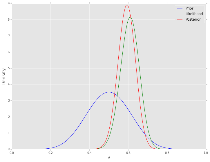
One simple way of numerical integration is to estimate the values on a grid of values for \(\theta\). To calculate the posterior, we find the prior and the likelhood for each value of \(\theta\), and for the marginal likelhood, we replace the integral with the equivalent sum
One advantage of this is that the prior does not have to be conjugate (although the example below uses the same beta prior for ease of comaprsion), and so we are not restricted in our choice of an approproirate prior distribution. For example, the prior can be a mixture distribution or estimated empirically from data. The disadvantage, of course, is that this is computationally very expenisve when we need to esitmate multiple parameters, since the number of grid points grows as \(\mathcal{O}(n^d)\), wher \(n\) defines the grid resolution and \(d\) is the size of \(\theta\).
thetas = np.linspace(0, 1, 200)
prior = st.beta(a, b)

post = prior.pdf(thetas) * st.binom(n, thetas).pmf(h)
post /= (post.sum() / len(thetas))

plt.figure(figsize=(12, 9))
plt.plot(thetas, prior.pdf(thetas), label='Prior', c='blue')
plt.plot(thetas, n*st.binom(n, thetas).pmf(h), label='Likelihood', c='green')
plt.plot(thetas, post, label='Posterior', c='red')
plt.xlim([0, 1])
plt.xlabel(r'$\theta$', fontsize=14)
plt.ylabel('Density', fontsize=16)
plt.legend();
Metropolis-Hastings sampler
This lecture will only cover the basic ideas of MCMC and the 3 common
veriants - Metropolis-Hastings, Gibbs and slice sampling. All ocde will
be built from the ground up to ilustrate what is involved in fitting an
MCMC model, but only toy examples will be shown since the goal is
conceptual understanding. More realiztic computational examples will be
shown in the next lecture using the pymc and pystan packages.
In Bayesian statistics, we want to estiamte the posterior distribution, but this is often intractable due to the high-dimensional integral in the denominator (marginal likelihood). A few other ideas we have encountered that are also relevant here are Monte Carlo integration with inddependent samples and the use of proposal distributions (e.g. rejection and importance sampling). As we have seen from the Monte Carlo inttegration lectures, we can approximate the posterior \(p(\theta | X)\) if we can somehow draw many samples that come from the posterior distribution. With vanilla Monte Carlo integration, we need the samples to be independent draws from the posterior distribution, which is a problem if we do not actually know what the posterior distribution is (because we cannot integrte the marginal likelihood).
With MCMC, we draw samples from a (simple) proposal distribution so that
each draw depends only on the state of the previous draw (i.e. the
samples form a Markov chain). Under certain condiitons, the Markov chain
will have a unique stationary distribution. In addition, not all samples
are used - instead we set up acceptance criteria for each draw based on
comparing successive states with respect to a target distribution that
enusre that the stationary distribution is the posterior distribution of
interest. The nice thing is that this target distribution only needs to
be proportional to the posterior distribution, which means we don’t need
to evaluate the potentially intractable marginal likelihood, which is
just a normalizing constant. We can find such a target distribution
easily, since posterior \(\propto\) likelihood
\(\times\) prior. After some time, the Markov chain of accepted
draws will converge to the staionary distribution, and we can use those
samples as (correlated) draws from the posterior distribution, and find
functions of the posterior distribution in the same way as for vanilla
Monte Carlo integration.
There are several flavors of MCMC, but the simplest to understand is the Metropolis-Hastings random walk algorithm, and we will start there.
To carry out the Metropolis-Hastings algorithm, we need to draw random samples from the folllowing distributions
- the standard uniform distribution
- a proposal distriution \(p(x)\) that we choose to be \(\mathcal{N}(0, \sigma)\)
- the target distribution \(g(x)\) which is proportional to the posterior probability
Given an initial guess for \(\theta\) with positive probability of being drawn, the Metropolis-Hastings algorithm proceeds as follows
Choose a new proposed value (\(\theta_p\)) such that \(\theta_p = \theta + \Delta\theta\) where \(\Delta \theta \sim \mathcal{N}(0, \sigma)\)
Caluculate the ratio
\[\rho = \frac{g(\theta_p \ | \ X)}{g(\theta \ | \ X)}\]where \(g\) is the posterior probability.
If the proposal distribution is not symmetrical, we need to weight the accceptanc probablity to maintain detailed balance (reversibilty) of the stationary distribution, and insetad calculate
\[\rho = \frac{g(\theta_p \ | \ X) p(\theta \ | \ \theta_p)}{g(\theta \ | \ X) p(\theta_p \ | \ \theta)}\]Since we are taking ratios, the denominator cancels any distribution proporational to \(g\) will also work - so we can use
\[\rho = \frac{p(X | \theta_p ) p(\theta_p)}{p(X | \theta ) p(\theta)}\]If \(\rho \ge 1\), then set \(\theta = \theta_p\)
If \(\rho < 1\), then set \(\theta = \theta_p\) with probability \(\rho\), otherwise set \(\theta = \theta\) (this is where we use the standard uniform distribution)
Repeat the earlier steps
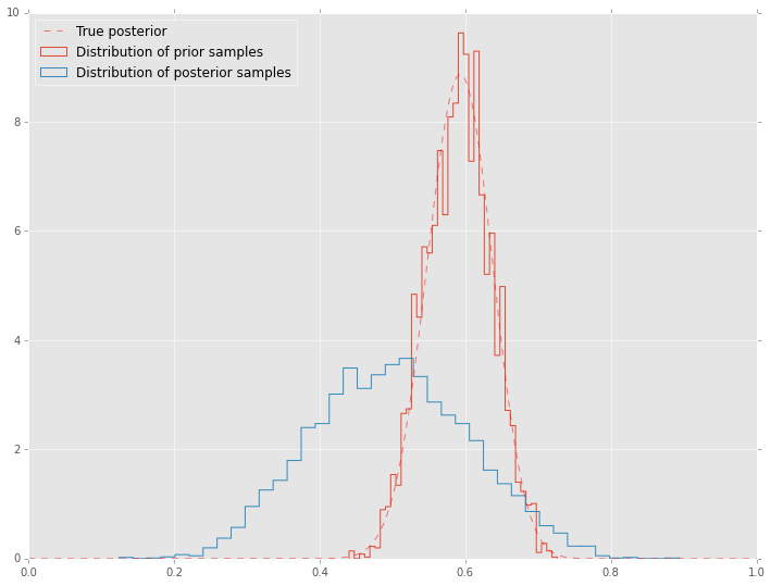
After some number of iterations \(k\), the samples \(\theta_{k+1}, \theta_{k+2}, \dots\) will be samples from the posterior distributions. Here are initial concepts to help your intuition about why this is so:
- We accept a proposed move to \(\theta_{k+1}\) whenever the density of the (unnormalzied) target distribution at \(\theta_{k+1}\) is larger than the value of \(\theta_k\) - so \(\theta\) will more often be found in places where the target distribution is denser
- If this was all we accepted, \(\theta\) would get stuck at a local mode of the target distribution, so we also accept occasional moves to lower density regions - it turns out that the correct probability of doing so is given by the ratio \(\rho\)
- The acceptance criteria only looks at ratios of the target distribution, so the denominator cancels out and does not matter - that is why we only need samples from a distribution proprotional to the posterior distribution
- So, \(\theta\) will be expected to bounce around in such a way that its spends its time in places proportional to the density of the posterior distribution - that is, \(\theta\) is a draw from the posterior distribution.
Additional notes:
Different propsoal distributions can be used for Metropolis-Hastings:
- The independence sampler uses a proposal distribtuion that is independent of the current value of \(\theta\). In this case the propsoal distribution needs to be similar to the posterior distirbution for efficincy, while ensuring that the acceptance ratio is bounded in the tail region of the posterior.
- The random walk sampler (used in this example) takes a random step centered at the current value of \(\theta\) - efficiecny is a trade-off between small step size with high probability of acceptance and large step sizes with low probaiity of acceptance. Note (picture will be sketched in class) that the random walk may take a long time to traverse narrow regions of the probabilty distribution. Changing the step size (e.g. scaling \(\Sigma\) for a multivariate normal proposal distribution) so that a target proportion of proposlas are accepted is known as tuning.
- Much research is being conducted on different proposal distributions for efficient sampling of the posterior distribution.
We will first see a numerical example and then try to understand why it works.
def target(lik, prior, n, h, theta):
    if theta < 0 or theta > 1:
        return 0
    else:
        return lik(n, theta).pmf(h)*prior.pdf(theta)

n = 100
h = 61
a = 10
b = 10
lik = st.binom
prior = st.beta(a, b)
sigma = 0.3

naccept = 0
theta = 0.1
niters = 10000
samples = np.zeros(niters+1)
samples[0] = theta
for i in range(niters):
    theta_p = theta + st.norm(0, sigma).rvs()
    rho = min(1, target(lik, prior, n, h, theta_p)/target(lik, prior, n, h, theta ))
    u = np.random.uniform()
    if u < rho:
        naccept += 1
        theta = theta_p
    samples[i+1] = theta
nmcmc = len(samples)//2
print "Efficiency = ", naccept/niters
Efficiency = 0.19
post = st.beta(h+a, n-h+b)

plt.figure(figsize=(12, 9))
plt.hist(samples[nmcmc:], 40, histtype='step', normed=True, linewidth=1, label='Distribution of prior samples');
plt.hist(prior.rvs(nmcmc), 40, histtype='step', normed=True, linewidth=1, label='Distribution of posterior samples');
plt.plot(thetas, post.pdf(thetas), c='red', linestyle='--', alpha=0.5, label='True posterior')
plt.xlim([0,1]);
plt.legend(loc='best');
Trace plots are often used to informally assess for stochastic convergence. Rigorous demonstration of convergence is an unsolved problem, but simple ideas such as running mutliple chains and checking that they are converging to similar distribtions are often employed in practice.
def mh_coin(niters, n, h, theta, lik, prior, sigma):
    samples = [theta]
    while len(samples) < niters:
        theta_p = theta + st.norm(0, sigma).rvs()
        rho = min(1, target(lik, prior, n, h, theta_p)/target(lik, prior, n, h, theta ))
        u = np.random.uniform()
        if u < rho:
            theta = theta_p
        samples.append(theta)
    return samples
n = 100
h = 61
lik = st.binom
prior = st.beta(a, b)
sigma = 0.05
niters = 100

sampless = [mh_coin(niters, n, h, theta, lik, prior, sigma) for theta in np.arange(0.1, 1, 0.2)]
# Convergence of multiple chains

for samples in sampless:
    plt.plot(samples, '-o')
plt.xlim([0, niters])
plt.ylim([0, 1]);

There are two main ideas - first that the samples generated by MCMC constitute a Markov chain, and that this Markov chain has a unique stationary distribution that is always reached if we geenrate a very large number of samples. The seocnd idea is to show that this stationary distribution is exactly the posterior distribution that we are looking for. We will only give the intuition here as a refreseher.
Since possible transitions depend only on the current and the proposed values of \(\theta\), the successive values of \(\theta\) in a Metropolis-Hastings sample consittute a Markov chain. Recall that for a Markov chain with a transition matrix \(P\)
means that \(\pi\) is a stationary distribution. If it is posssible to go from any state to any other state, then the matrix is irreducible. If in addtition, it is not possible to get stuck in an oscillation, then the matrix is also aperiodic or mixing. For finite state spaces, irreducibility and aperiodicity guarantee the existence of a unique stationary state. For continuous state space, we need an additional property of positive recurrence - starting from any state, the expected time to come back to the original state must be finitte. If we have all 3 peroperties of irreducibility, aperiodicity and positive recurrence, then there is a unique stationary distribution. The term ergodic is a little confusiong - most statndard definitinos take ergodicity to be equivalent to irreducibiltiy, but often Bayesian texts take ergoicity to mean irreducibility, aperiodicity and positive recurrence, and we wil follow the latter convention. For another intuitive perspective, the random walk Metropolish-Hasting algorithm is analogous to a diffusion process. Since all states are commmuicating (by design), eventually the system will settle into an equilibrium state. This is analaogous to converging on the stationary state.
We will considr the simplest possible scenario for an explicit
calculation. Suppose we have a two-state system where the posterior
probabilities are \(\theta\) and \(1 - \theta\). Suppose
\(\theta < 0.5\). So we have the following picture with the
Metropolish-Hastings algorithm:  and we find the
stationary distribution
\(\pi = \left( \begin{array}{cc} p & 1-p \end{array} \right)\) by
solving
to be \(\pi = \left( \begin{array}{cc} \theta & 1-\theta \end{array} \right)\), which is the posterior distribtion.
The final point is that a stationary distribution has to follow the detailed balance (reversibitily) criterion that says that the probability of being in state \(x\) and moving to state \(y\) must be the same as the probability of being in state \(y\) and moving to state \(x\). Or, more briefly,
and the need to make sure that this condition is true accounts for the strange looking acceptance criterion
Intuition
We want the stationary distribution \(\pi(x)\) to be the posterior distribution \(P(x)\). So we set
Rearranging, we get
We split the transition probability into separate proposal \(q\) and acceptance \(A\) parts, and after a little algebraic rearrangement get
An acceptance probability that meets this conidtion is
since \(A\) in the numerator and denominator are both bounded above by 1.
See http://www.cs.indiana.edu/~hauserk/downloads/MetropolisExplanation.pdf for algebraic details.
Gibbs sampler
Suppose we have a vector of parameters \(\theta = (\theta_1, \theta_2, \dots, \theta_k)\), and we want to estimate the joint posterior distribution \(p(\theta | X)\). Suppose we can find and draw random samples from all the conditional distributions
With Gibbs sampling, the Markov chain is constructed by sampling from the conditional distribution for each parameter \(\theta_i\) in turn, treating all other parameters as observed. When we have finished iterating over all parameters, we are said to have completed one cycle of the Gibbs sampler. Where it is difficult to sample from a conditional distribution, we can sample using a Metropolis-Hastings algorithm instead - this is known as Metropolis wihtin Gibbs.
Gibbs sampling is a type of random walk thorugh parameter space, and hence can be thought of as a Metroplish-Hastings algorithm with a special proposal distribtion. At each iteration in the cycle, we are drawing a proposal for a new value of a particular parameter, where the propsal distribution is the conditional posterior probability of that parameter. This means that the propsosal move is always accepted. Hence, if we can draw ssamples from the ocnditional distributions, Gibbs sampling can be much more efficient than regular Metropolis-Hastings.
Advantages of Gibbs sampling
- No need to tune proposal distribution
- Proposals are always accepted
Disadvantages of Gibbs sampling
- Need to be able to derive conditional probability distributions
- need to be able to draw random samples from contitional probability distributions
- Can be very slow if paramters are coorelated becauce you cannot take “diagonal” steps (draw picture to illustrate)
Motivating example
We will use the toy example of estimating the bias of two coins given sample pairs \((z_1, n_1)\) and \((z_2, n_2)\) where \(z_i\) is the number of heads in \(n_i\) tosses for coin \(i\).
Setup
def bern(theta, z, N):
    """Bernoulli likelihood with N trials and z successes."""
    return np.clip(theta**z * (1-theta)**(N-z), 0, 1)
def bern2(theta1, theta2, z1, z2, N1, N2):
    """Bernoulli likelihood with N trials and z successes."""
    return bern(theta1, z1, N1) * bern(theta2, z2, N2)
def make_thetas(xmin, xmax, n):
    xs = np.linspace(xmin, xmax, n)
    widths =(xs[1:] - xs[:-1])/2.0
    thetas = xs[:-1]+ widths
    return thetas
def make_plots(X, Y, prior, likelihood, posterior, projection=None):
    fig, ax = plt.subplots(1,3, subplot_kw=dict(projection=projection, aspect='equal'), figsize=(12,3))
    if projection == '3d':
        ax[0].plot_surface(X, Y, prior, alpha=0.3, cmap=plt.cm.jet)
        ax[1].plot_surface(X, Y, likelihood, alpha=0.3, cmap=plt.cm.jet)
        ax[2].plot_surface(X, Y, posterior, alpha=0.3, cmap=plt.cm.jet)
    else:
        ax[0].contour(X, Y, prior)
        ax[1].contour(X, Y, likelihood)
        ax[2].contour(X, Y, posterior)
    ax[0].set_title('Prior')
    ax[1].set_title('Likelihood')
    ax[2].set_title('Posteior')
    plt.tight_layout()
thetas1 = make_thetas(0, 1, 101)
thetas2 = make_thetas(0, 1, 101)
X, Y = np.meshgrid(thetas1, thetas2)
Analytic solution
a = 2
b = 3

z1 = 11
N1 = 14
z2 = 7
N2 = 14

prior = stats.beta(a, b).pdf(X) * stats.beta(a, b).pdf(Y)
likelihood = bern2(X, Y, z1, z2, N1, N2)
posterior = stats.beta(a + z1, b + N1 - z1).pdf(X) * stats.beta(a + z2, b + N2 - z2).pdf(Y)
make_plots(X, Y, prior, likelihood, posterior)
make_plots(X, Y, prior, likelihood, posterior, projection='3d')


Grid approximation
def c2d(thetas1, thetas2, pdf):
    width1 = thetas1[1] - thetas1[0]
    width2 = thetas2[1] - thetas2[0]
    area = width1 * width2
    pmf = pdf * area
    pmf /= pmf.sum()
    return pmf
_prior = bern2(X, Y, 2, 8, 10, 10) + bern2(X, Y, 8, 2, 10, 10)
prior_grid = c2d(thetas1, thetas2, _prior)
_likelihood = bern2(X, Y, 1, 1, 2, 3)
posterior_grid = _likelihood * prior_grid
posterior_grid /= posterior_grid.sum()
make_plots(X, Y, prior_grid, likelihood, posterior_grid)
make_plots(X, Y, prior_grid, likelihood, posterior_grid, projection='3d')


Metropolis
a = 2
b = 3

z1 = 11
N1 = 14
z2 = 7
N2 = 14

prior = lambda theta1, theta2: stats.beta(a, b).pdf(theta1) * stats.beta(a, b).pdf(theta2)
lik = partial(bern2, z1=z1, z2=z2, N1=N1, N2=N2)
target = lambda theta1, theta2: prior(theta1, theta2) * lik(theta1, theta2)

theta = np.array([0.5, 0.5])
niters = 10000
burnin = 500
sigma = np.diag([0.2,0.2])

thetas = np.zeros((niters-burnin, 2), np.float)
for i in range(niters):
    new_theta = stats.multivariate_normal(theta, sigma).rvs()
    p = min(target(*new_theta)/target(*theta), 1)
    if np.random.rand() < p:
        theta = new_theta
    if i >= burnin:
        thetas[i-burnin] = theta
kde = stats.gaussian_kde(thetas.T)
XY = np.vstack([X.ravel(), Y.ravel()])
posterior_metroplis = kde(XY).reshape(X.shape)
make_plots(X, Y, prior(X, Y), lik(X, Y), posterior_metroplis)
make_plots(X, Y, prior(X, Y), lik(X, Y), posterior_metroplis, projection='3d')


Gibbs
a = 2
b = 3

z1 = 11
N1 = 14
z2 = 7
N2 = 14

prior = lambda theta1, theta2: stats.beta(a, b).pdf(theta1) * stats.beta(a, b).pdf(theta2)
lik = partial(bern2, z1=z1, z2=z2, N1=N1, N2=N2)
target = lambda theta1, theta2: prior(theta1, theta2) * lik(theta1, theta2)

theta = np.array([0.5, 0.5])
niters = 10000
burnin = 500
sigma = np.diag([0.2,0.2])

thetas = np.zeros((niters-burnin,2), np.float)
for i in range(niters):
    theta = [stats.beta(a + z1, b + N1 - z1).rvs(), theta[1]]
    theta = [theta[0], stats.beta(a + z2, b + N2 - z2).rvs()]

    if i >= burnin:
        thetas[i-burnin] = theta
kde = stats.gaussian_kde(thetas.T)
XY = np.vstack([X.ravel(), Y.ravel()])
posterior_gibbs = kde(XY).reshape(X.shape)
make_plots(X, Y, prior(X, Y), lik(X, Y), posterior_gibbs)
make_plots(X, Y, prior(X, Y), lik(X, Y), posterior_gibbs, projection='3d')


Slice sampler
Yet another MCMC algorithm is slice sampling. In slice sampling, the Markov chain is constructed by using an auxiliary variable representing slices throuth the (unnomrmalized) posterior distribution that is constructed using only the current parmater value. Like Gibbs sampling, there is no tuning processs and all proposals are accepted. For slice sampling, you either need the inverse distibution function or some way to estimate it.
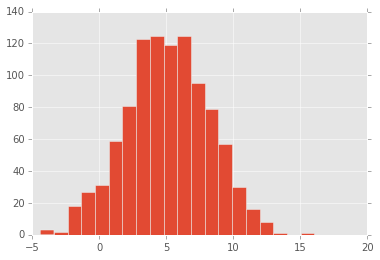
A toy example illustrates the process - Suppose we want to draw random samples from the posterior distribution \(\mathcal{N}(0, 1)\) using slice sampling
Start with some value \(x\) - sample \(y\) from \(\mathcal{U}(0, f(x))\) - this is the horizontal “slice” that gives the method its name - sample the next \(x\) from \(f^{-1}(y)\) - this is typicaly done numerically - repeat
# Code illustrating idea of slice sampler

import scipy.stats as stats

dist = stats.norm(5, 3)
w = 0.5
x = dist.rvs()

niters = 1000
xs = []
while len(xs) < niters:
    y = np.random.uniform(0, dist.pdf(x))
    lb = x
    rb = x
    while y < dist.pdf(lb):
        lb -= w
    while y < dist.pdf(rb):
        rb += w
    x = np.random.uniform(lb, rb)
    if y > dist.pdf(x):
        if np.abs(x-lb) < np.abs(x-rb):
            lb = x
        else:
            lb = y
    else:
        xs.append(x)
plt.hist(xs, 20);
Notes on the slice sampler:
- the slice may consist of disjoint pieces for multimodal distribtuions
- the slice can be a rectangular hyperslab for multivariable posterior distributions
- sampling from the slice (i.e. finding the boundaries at level \(y\)) is non-trivial and may involve iterative rejection steps - see figure below from Wikipedia for a typical approach - the blue bars represent disjoint pieces of the true slice through a bimodal distribution and the black lines are the proposal distribution approximaitng the true slice
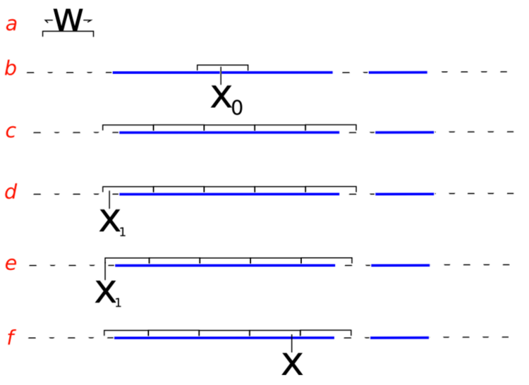
Slice sampling algorithm from Wikipedia
Hierarchical models
Hierarchical models have the following structure - first we specify that the data come from a distribution with parameers \(\theta\)
and that the parameters themselves come from anohter distribution with hyperparameters \(\lambda\)
and finally that \(\lambda\) comes from a prior distribution
More levels of hiearchy are possible - i.e you can specify hyper-hyperparameters for the dsitribution of \(\lambda\) and so on.
The essential idea of the hierarchical model is because the \(\theta\)s are not independent but rather are drawen from a common distribution with parameter \(\lambda\), we can share information across the \(\theta\)s by also estimating \(\lambda\) at the same time.
As an example, suppose have data about the proportion of heads after some number of tosses from several coins, and we want to estimate the bias of each coin. We also know that the coins come from the same mint and so might share soem common manufacturing defect. There are two extreme apporaches - we could estimate the bias of each coin from its coin toss data independently of all the others, or we could pool the results together and estimate the same bias for all coins. Hiearchical models proivde a compromise where we shrink individual estiamtes towards a common estimate.
Note that because of the conditionally indpeendent structure of hiearchical models, Gibbs sampling is often a natural choice for the MCMC sampling strategy.
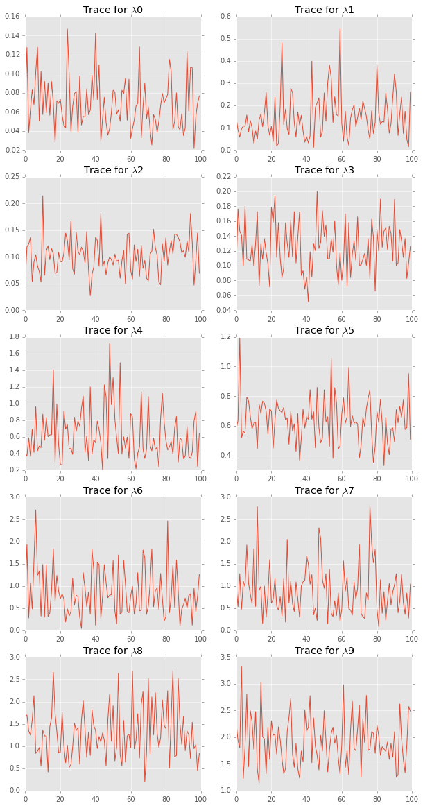
Suppose we have data of the number of failures (\(y_i\)) for each of 10 pumps in a nuclear plant. We also have the times (\(_i\)) at which each pump was observed. We want to model the number of failures with a Poisson likelihood, where the expected number of failure \(\lambda_i\) differs for each pump. Since the time which we observed each pump is different, we need to scale each \(\lambda_i\) by its observed time \(t_i\).
We now specify the hiearchcical model - note change of notation from the overview above - that \(\theta\) is \(\lambda\) (parameter) and \(\lambda\) is \(\beta\) (hyperparameter) simply because \(\lambda\) is traditional for the Poisson distribution parameter.
The likelihood \(f\) is
We let the prior \(g\) for \(\lambda\) be
with \(\alpha = 1.8\) (an improper prior whose integral does not sum to 1)
and let the hyperprior \(h\) for \(\beta\) to be
with \(\gamma = 0.01\) and \(\delta = 1\).
There are 11 unknown parameters (10 \(\lambda\)s and \(\beta\)) in this hierarchical model.
The posterior is
with the condiitonal distributions needed for Gibbs sampling given by
and
from numpy.random import gamma as rgamma # rename so we can use gamma for parameter name
def lambda_update(alpha, beta, y, t):
    return rgamma(size=len(y), shape=y+alpha, scale=1.0/(t+beta))

def beta_update(alpha, gamma, delta, lambd, y):
    return rgamma(size=1, shape=len(y) * alpha + gamma, scale=1.0/(delta + lambd.sum()))

def gibbs(niter, y, t, alpha, gamma, delta):
    lambdas_ = np.zeros((niter, len(y)), np.float)
    betas_ = np.zeros(niter, np.float)

    lambda_ = y/t

    for i in range(niter):
        beta_ = beta_update(alpha, gamma, delta, lambda_, y)
        lambda_ = lambda_update(alpha, beta_, y, t)

        betas_[i] = beta_
        lambdas_[i,:] = lambda_

    return betas_, lambdas_
alpha = 1.8
gamma = 0.01
delta = 1.0
beta0 = 1
y = np.array([5, 1, 5, 14, 3, 19, 1, 1, 4, 22], np.int)
t = np.array([94.32, 15.72, 62.88, 125.76, 5.24, 31.44, 1.05, 1.05, 2.10, 10.48], np.float)
niter = 1000
betas, lambdas = gibbs(niter, y, t, alpha, gamma, delta)
print '%.3f' % betas.mean()
print '%.3f' % betas.std(ddof=1)
print lambdas.mean(axis=0)
print lambdas.std(ddof=1, axis=0)
2.469
0.692
[ 0.0697  0.1557  0.1049  0.1236  0.6155  0.619   0.809   0.8304  1.2989
  1.8404]
[ 0.027   0.0945  0.0396  0.0305  0.2914  0.1355  0.5152  0.529   0.57
  0.391 ]
plt.figure(figsize=(10, 20))
for i in range(len(lambdas.T)):
    plt.subplot(5,2,i+1)
    plt.plot(lambdas[::10, i]);
    plt.title('Trace for $\lambda$%d' % i)
LaTeX for Markov chain diagram
documentclass[10pt]{article} usepackage[usenames]{color} usepackage{amssymb} usepackage{amsmath} usepackage[utf8]{inputenc} usepackage {tikz} usetikzlibrary{automata,arrows,positioning}
begin{tikzpicture}[->,>=stealth’,shorten >=1pt,auto,node distance=2.8cm, semithick] tikzstyle{every state}=[fill=white,draw=black,thick,text=black,scale=1] node[state] (A) {$theta$}; node[state] (B) [right of=A] {$1-theta$}; path (A) edge [bend left] node[above] {$1$} (B); path (B) edge [bend left] node[below] {$frac{theta}{1-theta}$} (A); path (A) edge [loop above] node {0} (A); path (B) edge [loop above] node {$1-frac{theta}{1-theta}$} (B); end{tikzpicture}