Unsupervised and Supervised Learning
In [2]:
library(tidyverse)
Loading tidyverse: ggplot2
Loading tidyverse: tibble
Loading tidyverse: tidyr
Loading tidyverse: readr
Loading tidyverse: purrr
Loading tidyverse: dplyr
Conflicts with tidy packages ---------------------------------------------------
filter(): dplyr, stats
lag():    dplyr, stats
In [24]:
library(pheatmap)
In [3]:
options(repr.plot.width=6, repr.plot.height=6)
Toy data set
In [4]:
head(iris)
| Sepal.Length | Sepal.Width | Petal.Length | Petal.Width | Species |
|---|---|---|---|---|
| 5.1 | 3.5 | 1.4 | 0.2 | setosa |
| 4.9 | 3.0 | 1.4 | 0.2 | setosa |
| 4.7 | 3.2 | 1.3 | 0.2 | setosa |
| 4.6 | 3.1 | 1.5 | 0.2 | setosa |
| 5.0 | 3.6 | 1.4 | 0.2 | setosa |
| 5.4 | 3.9 | 1.7 | 0.4 | setosa |
Note: If you want graphics based on ggplot2, install the
`GGally <https://cran.r-project.org/web/packages/GGally/index.html>`__
package and use the ggpairs function. This has not been installed on
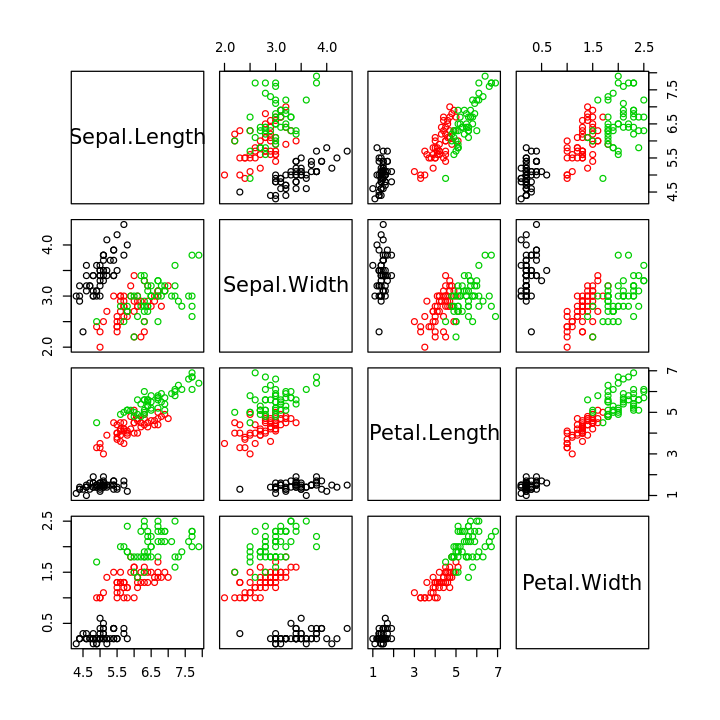
the OIT Docker containers, so we use the simpler pairs function from
base graphics.
library(GGally)
ggpairs(iris, aes(colour = Species))
In [5]:
pairs(iris[,1:4], col=iris$Species)
Unsupervised Learning
Ordination (Dimension reduction)
PCA
In [6]:
pca <- as.data.frame(prcomp(iris[,1:4], center=TRUE, scale=TRUE, rank=2)$x)
In [7]:
dim(pca)
- 150
- 2
In [8]:
pca <- bind_cols(iris, pca)
In [9]:
head(pca)
| Sepal.Length | Sepal.Width | Petal.Length | Petal.Width | Species | PC1 | PC2 |
|---|---|---|---|---|---|---|
| 5.1 | 3.5 | 1.4 | 0.2 | setosa | -2.257141 | -0.4784238 |
| 4.9 | 3.0 | 1.4 | 0.2 | setosa | -2.074013 | 0.6718827 |
| 4.7 | 3.2 | 1.3 | 0.2 | setosa | -2.356335 | 0.3407664 |
| 4.6 | 3.1 | 1.5 | 0.2 | setosa | -2.291707 | 0.5953999 |
| 5.0 | 3.6 | 1.4 | 0.2 | setosa | -2.381863 | -0.6446757 |
| 5.4 | 3.9 | 1.7 | 0.4 | setosa | -2.068701 | -1.4842053 |
In [10]:
options(repr.plot.width=5.5, repr.plot.height=4)
In [11]:
ggplot(pca, aes(x=PC1, y=PC2, color=Species)) +
geom_point()
Data type cannot be displayed:

MDS
In [12]:
dist(iris[1:5,1:4])
1         2         3         4
2 0.5385165
3 0.5099020 0.3000000
4 0.6480741 0.3316625 0.2449490
5 0.1414214 0.6082763 0.5099020 0.6480741
In [13]:
mds <- as.data.frame(cmdscale(dist(iris[,1:4]), k = 2))
In [14]:
dim(mds)
- 150
- 2
In [15]:
mds <- bind_cols(mds, iris)
In [16]:
head(mds)
| V1 | V2 | Sepal.Length | Sepal.Width | Petal.Length | Petal.Width | Species |
|---|---|---|---|---|---|---|
| -2.684126 | 0.3193972 | 5.1 | 3.5 | 1.4 | 0.2 | setosa |
| -2.714142 | -0.1770012 | 4.9 | 3.0 | 1.4 | 0.2 | setosa |
| -2.888991 | -0.1449494 | 4.7 | 3.2 | 1.3 | 0.2 | setosa |
| -2.745343 | -0.3182990 | 4.6 | 3.1 | 1.5 | 0.2 | setosa |
| -2.728717 | 0.3267545 | 5.0 | 3.6 | 1.4 | 0.2 | setosa |
| -2.280860 | 0.7413304 | 5.4 | 3.9 | 1.7 | 0.4 | setosa |
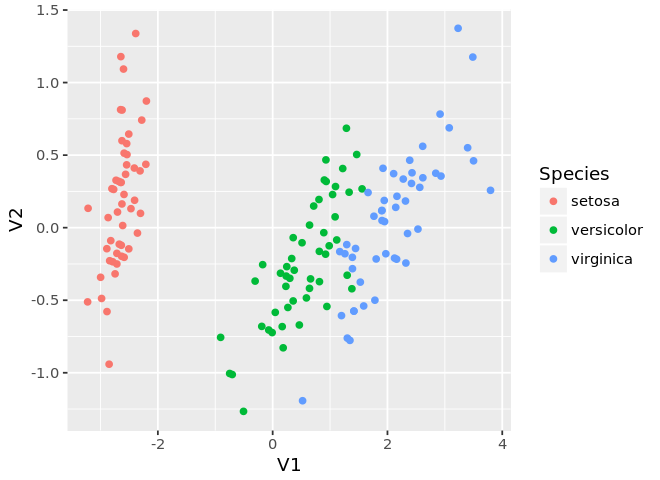
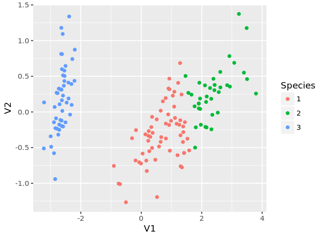
In [17]:
ggplot(mds, aes(x=V1, y=V2, color=Species)) +
geom_point()
Data type cannot be displayed:
Clustering
Note: If you want graphics based on ggplot2, install the
`gdendro <https://cran.r-project.org/web/packages/ggdendro/vignettes/ggdendro.html>`__
package and use the ggdendrogram function. This has not been
installed on the OIT Docker containers, so we use the simpler plot
function from base graphics.
hc <- hclust(dist(iris[,1:4]), 'complete')
ggdendrogram(hc, rotate = FALSE, size = 2)
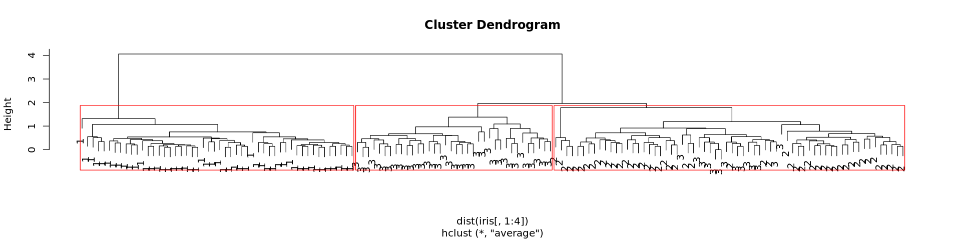
Agglomertive clustering
In [18]:
options(repr.plot.width=16, repr.plot.height=4)
In [19]:
tree <- hclust(dist(iris[,1:4]), method='average')
In [20]:
tree$labels <- as.integer(iris$Species)
In [21]:
plot(tree)

In [22]:
plot(tree)
rect.hclust(tree, k=3, border = "red")
Dendrograms are also constructed as part of visualizing a heatmapm
In [33]:
?pheatmap
In [29]:
options(repr.plot.width=5, repr.plot.height=6)
In [32]:
pheatmap(iris[,1:4], show_rownames = FALSE)

Visualize clusters on MDS plot
In [23]:
ggplot(mds, aes(x=V1, y=V2, color=Species)) +
geom_point() +
guides(color=guide_legend(title='Species'))
Data type cannot be displayed:

In [24]:
z <- cutree(tree, k = 3)
In [25]:
ggplot(mds, aes(x=V1, y=V2, color=as.factor(z))) +
geom_point() +
guides(color=guide_legend(title='Species'))
Data type cannot be displayed:

K-means clustering
In [26]:
km <- kmeans(iris[,1:4], centers=3)
In [27]:
km
K-means clustering with 3 clusters of sizes 62, 38, 50

Cluster means:
  Sepal.Length Sepal.Width Petal.Length Petal.Width
1     5.901613    2.748387     4.393548    1.433871
2     6.850000    3.073684     5.742105    2.071053
3     5.006000    3.428000     1.462000    0.246000

Clustering vector:
  [1] 3 3 3 3 3 3 3 3 3 3 3 3 3 3 3 3 3 3 3 3 3 3 3 3 3 3 3 3 3 3 3 3 3 3 3 3 3
 [38] 3 3 3 3 3 3 3 3 3 3 3 3 3 1 1 2 1 1 1 1 1 1 1 1 1 1 1 1 1 1 1 1 1 1 1 1 1
 [75] 1 1 1 2 1 1 1 1 1 1 1 1 1 1 1 1 1 1 1 1 1 1 1 1 1 1 2 1 2 2 2 2 1 2 2 2 2
[112] 2 2 1 1 2 2 2 2 1 2 1 2 1 2 2 1 1 2 2 2 2 2 1 2 2 2 2 1 2 2 2 1 2 2 2 1 2
[149] 2 1

Within cluster sum of squares by cluster:
[1] 39.82097 23.87947 15.15100
 (between_SS / total_SS =  88.4 %)

Available components:

[1] "cluster"      "centers"      "totss"        "withinss"     "tot.withinss"
[6] "betweenss"    "size"         "iter"         "ifault"
Visualize clusters on MDS plot
In [28]:
ggplot(mds, aes(x=V1, y=V2, color=Species)) +
geom_point() +
guides(color=guide_legend(title='Species'))
Data type cannot be displayed:

In [29]:
ggplot(mds, aes(x=V1, y=V2, color=as.factor(km$cluster))) +
geom_point() +
guides(color=guide_legend(title='Species'))
Data type cannot be displayed:
Supervised Learning
If you need to tune the model parameters, you will need to construct an additional validation data set.
In [30]:
idx <- sample(1:nrow(iris), 50)
In [31]:
idx
- 113
- 57
- 22
- 141
- 94
- 140
- 44
- 103
- 62
- 29
- 16
- 41
- 87
- 8
- 53
- 146
- 21
- 46
- 3
- 18
- 150
- 15
- 25
- 60
- 109
- 38
- 34
- 130
- 81
- 144
- 26
- 19
- 80
- 96
- 40
- 121
- 92
- 119
- 27
- 11
- 75
- 149
- 114
- 20
- 129
- 73
- 137
- 14
- 47
- 51
In [32]:
iris.test <- iris[idx,]
iris.train <- iris[-idx,]
In [33]:
library(nnet)
In [34]:
fit <- multinom(Species ~ ., data=iris.train)
# weights:  18 (10 variable)
initial  value 109.861229
iter  10 value 9.488101
iter  20 value 5.718048
iter  30 value 5.607010
iter  40 value 5.566651
iter  50 value 5.564816
iter  60 value 5.559930
final  value 5.559325
converged
In [35]:
fit
Call:
multinom(formula = Species ~ ., data = iris.train)

Coefficients:
           (Intercept) Sepal.Length Sepal.Width Petal.Length Petal.Width
versicolor    15.30068    -4.714006   -8.950189     12.66693    2.132277
virginica    -19.12182    -6.891088  -15.500148     20.84077   18.004415

Residual Deviance: 11.11865
AIC: 31.11865
In [36]:
pred <- predict(fit, newdata = iris.test)
In [37]:
mds.test <- mds[idx,]
In [38]:
ggplot(mds.test, aes(x=V1, y=V2, color=as.factor(pred))) +
geom_point() +
guides(color=guide_legend(title='Species')) +
labs(title='Observed')
Data type cannot be displayed:

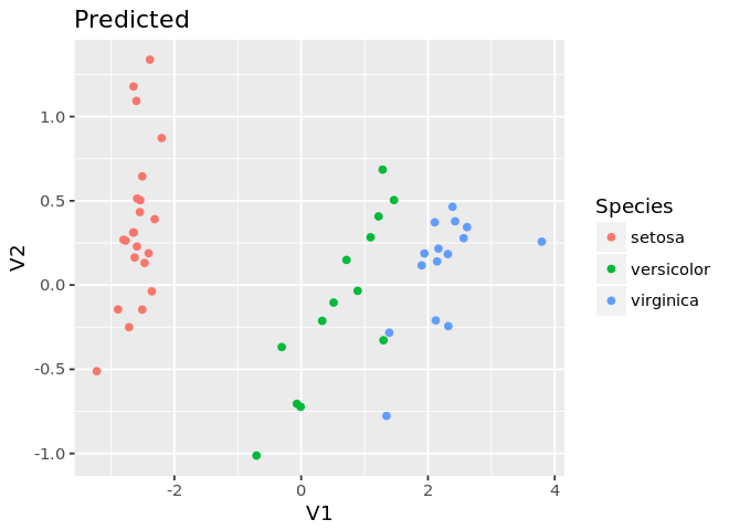
In [39]:
ggplot(mds.test, aes(x=V1, y=V2, color=as.factor(Species))) +
geom_point() +
guides(color=guide_legend(title='Species')) +
labs(title='Predicted')
Data type cannot be displayed: