Constructed Climates

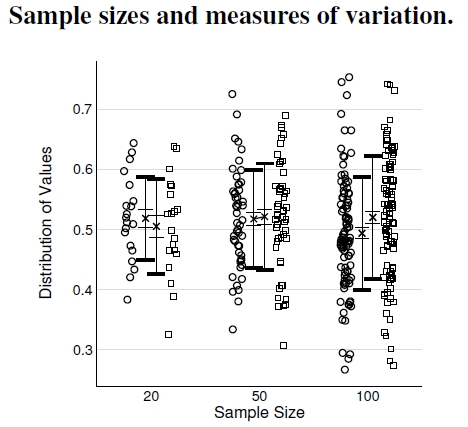
Figure A.6: A fundamental difference exists between a distribution’s standard deviation and the standard error in a sample of points. Circles and squares arise from two distributions having the same standard deviation, 0.1, but different means, 0.49 and 0.51, respectively. Sampling just 20 points from each distribution results in rather poor estimates of the standard deviation, given by the thick bars, and overlapping standard errors, the thin bars, that do not resolve the differences between the distributions’ means. Increasing the sample sizes to 50 and 100 provide better estimates of the standard deviations, and the standard errors shrink enough to distinguish the differing means.

Imagine some process that has an outcome governed partly by chance and partly by mechanisms. Something more complicated than just a coin flip with a heads or tails outcome, more like flipping 100 coins, which, on average would produce 50 heads and 50 tails. A distribution of outcomes like that one has a mean, or average value, and some width, like a bell curve. A standard deviation—which mustn’t be confused with a study’s standard error (explained below) — provides the most common measure of the distribution’s width. If a scientist undertakes a single measurement from an experiment whose outcome follows a particular distribution, about 68% of the time the experiment’s result will fall between the mean minus the standard deviation and the mean plus the standard deviation.

I produced my figure here using a computer program to sample two different “normal” distributions[5], and again think bell curves. My distributions, which I’ve plotted as circles and squares, have slightly different means, 0.49 and 0.51, respectively, and identical standard deviations, 0.1.[6]

The standard deviation of a distribution is very different from the standard error in a sample of measurements. The former involves the width of the distribution and the latter estimates how accurately an experiment estimates the distribution’s mean. In the figure I show, between (and alongside) the circles and squares for each set, the averages, standard errors, and standard deviations. Each “x” marks the sample average, the thinner error bars closest to the x delimit the standard error, and the thicker error bars at the ends mark the standard deviation.

First, notice how the standard deviation error bars change length between sample sizes 20 and 50, but hardly at all between sample sizes 50 and 100. Experiments with large sample sizes provide good estimates of the underlying distributions, at least as measured by distribution width.

Second, standard errors decrease as an experiment’s sample size increases. Statisticians proved that an experiment’s standard error equals the underlying distribution’s standard deviation divided by √N, where N equals the sample size. Given this connection, quadrupling the sample size only halves the standard error.

Third, the standard error represents how accurately an experiment estimates the distribution’s mean. For example, compare the means and standard errors from the N = 20 experiment with the those of the N = 100 experiment. Small sample size experiments don’t estimate means terribly well, but their standard errors cover the actual means, well-estimated by the large sample size experiment.

Finally, scientists invoke statistical tests to decide whether two averages differ; for example, are there different social benefits in barren versus green environments? These tests try to distinguish differences between the estimated averages for the N = 20 experiment, where detection is impossible, and the N = 100 experiment, where the difference is clear.

—————————-

[5]Normal distributions are a more technical name for the “bell-curves” sometimes mentioned more informally. They also go by the name Gaussian distribution. I could show the formula, but more complete descriptions can be found elsewhere because they’re so normal.

[6]I gave both distributions the same standard deviation, 0.1, meaning roughly 68% of the points will fall between 0.39 (0.41) and 0.59 (0.61), verified by the really dark region in those bands for the high sample size example.