Notes on linear
regression analysis (pdf file)
Introduction to linear
regression analysis
Mathematics
of simple regression
Regression examples
·
Beer sales vs. price, part 1: descriptive
analysis
·
Beer sales vs. price, part 2: fitting a simple
model
·
Beer sales vs.
price, part 3: transformations of variables
·
Beer sales vs.
price, part 4: additional predictors
·
NC natural gas
consumption vs. temperature
·
More regression datasets
at regressit.com
What to
look for in regression output
What’s a good value for R-squared?
What's the bottom line? How to compare models
Testing the assumptions of linear regression
Additional notes on regression analysis
Stepwise and all-possible-regressions
Excel file with
simple regression formulas
Excel file with regression
formulas in matrix form
Notes on logistic regression (new!)
If you use
Excel in your work or in your teaching to any extent, you should check out the latest
release of RegressIt, a free Excel add-in for linear and logistic regression.
See it at regressit.com. The linear regression version runs on both PC's and Macs and
has a richer and easier-to-use interface and much better designed output than
other add-ins for statistical analysis. It may make a good complement if not a
substitute for whatever regression software you are currently using,
Excel-based or otherwise. RegressIt is an excellent tool for interactive
presentations, online teaching of regression, and development of videos of
examples of regression modeling. It includes extensive built-in
documentation and pop-up teaching notes as well as some novel features to
support systematic grading and auditing of student work on a large scale. There
is a separate logistic
regression version with
highly interactive tables and charts that runs on PC's. RegressIt also now
includes a two-way
interface with R that allows
you to run linear and logistic regression models in R without writing any code
whatsoever.
If you have
been using Excel's own Data Analysis add-in for regression (Analysis Toolpak),
this is the time to stop. It has not
changed since it was first introduced in 1993, and it was a poor design even
then. It's a toy (a clumsy one at that), not a tool for serious work. Visit
this page for a discussion: What's wrong with Excel's Analysis Toolpak for regression
Regression
example, part 3: transformations of
variables
In the beer sales example, a simple regression fitted to the original variables
(price-per-case and cases-sold
for 18-packs) yields poor results because it makes wrong assumptions about the
nature of the patterns in the data.
The relationship between the two variables is not linear, and if a
linear model is fitted anyway, the errors do not have the distributional
properties that a regression model assumes, and forecasts and lower confidence
limits at the upper end of the price range have negative values. What to do in such a case? In some situations there may be omitted
variables which, if they could be identified and added to the model, would
correct the problems. In other
situations it could be that breaking the data set up into subsets, on the basis
of ranges of the independent variables, would allow linear models to fit
reasonably well. And there are more
complex model types that could be tried--linear regression models are merely
the simplest place to start. But an
often-used and often-successful strategy is to look for transformations of the original variables that straighten out the
curves, normalize the errors, and/or exploit the time dimension.
In modeling consumer demand, a standard
approach is to apply a natural log
transformation to both prices and quantities before fitting a regression
model. As was discussed on the log transformation page in these notes, when a simple linear regression model
is fitted to logged variables, the slope coefficient represents the predicted percent change in the dependent variable
per percent change in the independent
variable, regardless of their current levels. Larger changes in the independent
variable are predicted to result in a compounding
of the marginal effects rather than a linear extrapolation of them. Let’s see how this approach works
on the beer sales data.
Suppose that we apply a natural log
transformation to all 6 of the price and sales variables in the data set, and
let the names of the logged variables be the original variables with
“_LN” appended to them.
(This is the naming convention used by the variable-transformation tool
in RegressIt.) The
correlation matrix and scatterplot matrix of of the logged variables look like
this:
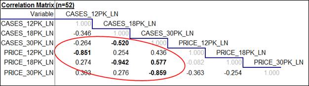
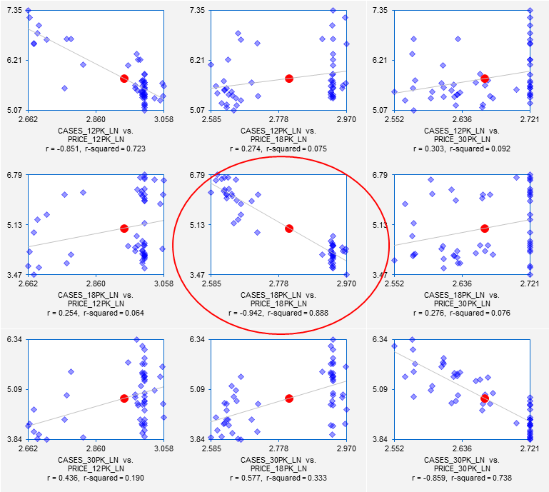
The correlations are slightly stronger
among the logged variables than among the original variables, and the variance
of the vertical deviations from the regression lines in the scatterplots is now
very similar for both large and small values of the horizontal-axis
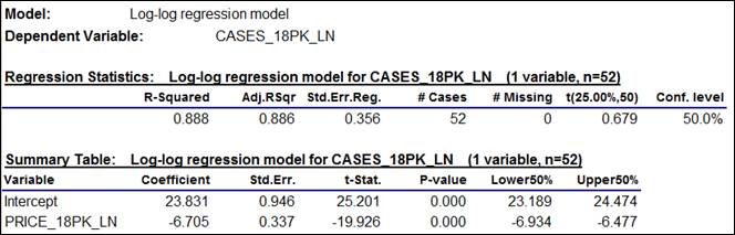
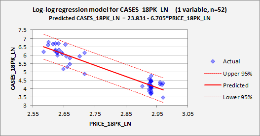
variable. So, let us try fitting a
simple regression model to the logged 18-pack variables. The summary table for the model is shown
below. The slope coefficient of
-6.705 means that on the margin a 1%
change in price is predicted to lead to a 6.7% change in sales, in the opposite
direction, with a compounding of this effect for larger percentage price
changes. The standard error of the
regression of 0.356 is not directly comparable to that of the original model,
because it is measured in log units.
(Return to top of page.)
If the standard error of the regression
in a model fitted to logged data is on the order of 0.1 or less, it can be
roughly interpreted as the standard error of a forecast measured in percentage
terms. For example, if the standard
error of the regression was 0.05, it would be OK to say that the standard error
of a forecast is about 5% of the forecast value. (An increase of 0.05 in the
natural log of variable corresponds to a proportional change of LN(1.05) ≈
0.049, or 4.9%, and a decrease of 0.05 in the natural log corresponds to a
proportional change of LN(0.95) ≈ -0.051, or -5.1%, so +/- 0.05 in log
units is about the same as +/-5% in percentage terms. For a change of +/- 0.1 in the natural
log, the corresponding proportional changes are LN(1.1) ≈ .105 and
LN(0.9) ≈ 0.095, i.e., +10.5% or -9.5%, and so on.) The regression
standard error of 0.356 observed here is too large for that approximation to
apply, i.e., it would not be NOT be OK to say that the standard error of a
forecast is 36% of the forecast value, because the confidence limits are not
sufficiently symmetric around the point forecast. However, this does indicate that the
unexplained variations in demand are fairly large in percentage terms.
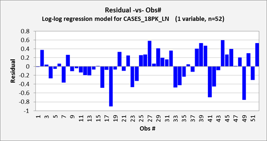
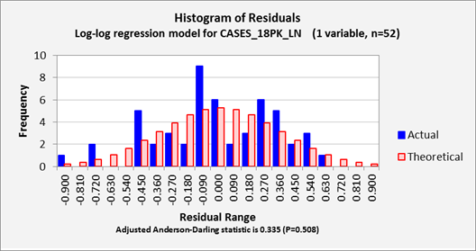
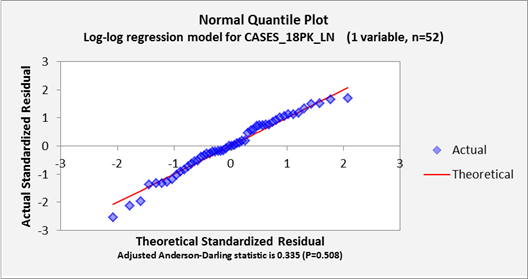
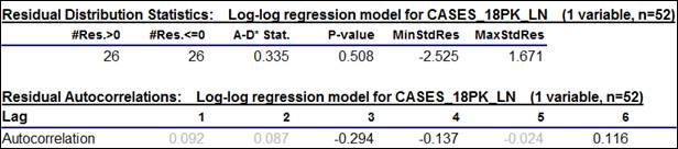
The residual statistics table shows that
the distribution of the errors is very close to a normal distribution (the A-D*
stat is very small, with a P-value on the order of 0.5), and the
autocorrelations of the errors are insignificant at the first couple of
lags. (Unless we are looking for
seasonal patterns, we usually are only concerned with the first couple of lags
as far as autocorrelations are concerned.)
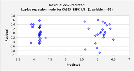
The line fit plot also looks very
good: the vertical deviations from
the regression line are approximately the same size for large and small predictions,
and they nicely fill the space between the 95% confidence limits.
The rest of the chart output of the model
is shown farther down on this page, and it all looks reasonably good, so I will
not discuss it further. What is of special interest is the
appearance of the forecasts that are generated by this model when they are
translated from log units back into real units of cases. This requires applying the EXP
function to the forecasts and their lower and upper confidence limits generated
by the log-log model. (Return to top of page.)
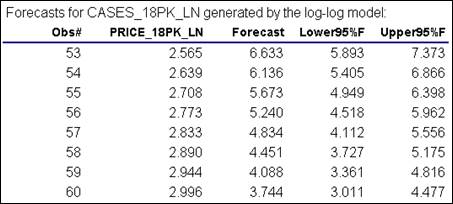
All regression software has the
capability to generate forecasts for additional values of the independent
variables provided by the user.
Often the convention is for the program to automatically generate forecasts for any rows of data where the
independent variables are all present and the dependent variable is
missing. That convention is
followed in RegressIt. Here,
forecasts for log sales have been automatically generated for integer-valued
prices in the range from $13 to $20 (numbers that are just outside the
historical minimum and maximum), which were included in the original data
file.
Here are the results of applying the EXP
function to the numbers in the table above to convert them back to real units:
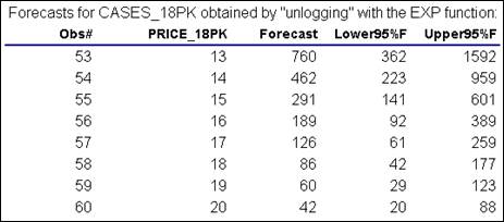
Note that all the numbers are positive,
and the widths of the confidence intervals are proportional to the size of the
forecasts. They are not symmetric,
though: they are wider on the high
side than the low side, which is logical.
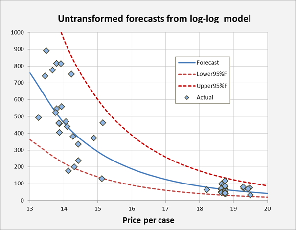
Here’s a chart generated from the last table, which tells the
story: the nonlinear forecast curve
captures the steeper slope of the pattern in the data at low price levels, and
the confidence limits fit the magnitudes of random variations at both low and
high price levels.
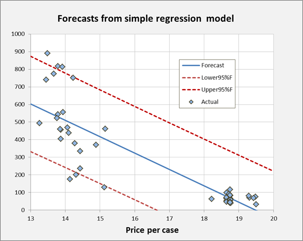
For purposes of comparison, here is a
similarly formatted chart of forecasts produced by the original regression
model for unlogged data. Which
looks more reasonable?
The rest of the chart output from the
log-log model is shown farther down on this page, and it looks fine as
regression models go. The
take-aways from this step of the analysis are the following:
·
The log-log model is well
supported by economic theory and it does a very plausible job of fitting the
price-demand pattern in the beer sales data.
·
The nonlinear curve in the
(unlogged) forecasts adapts to the steeper slope in the demand function at low
price levels.
·
The way in which the width
of the confidence intervals scales in proportion to the forecasts provides a
good fit to the vertical distribution of sales values at different price
levels.
·
It is impossible for the
log-log model’s forecasts or confidence limits for real sales to be
negative.
There is more to be done with this
analysis, namely considering the effects of other variables. Click here to proceed to that step.