Notes on linear
regression analysis (pdf file)
Introduction
to linear regression analysis
Mathematics
of simple regression
Regression examples
·
Beer sales vs. price, part 1: descriptive
analysis
·
Beer sales vs. price, part 2: fitting a simple
model
·
Beer sales vs. price, part 3: transformations
of variables
·
Beer sales vs.
price, part 4: additional predictors
·
NC natural gas
consumption vs. temperature
·
More regression datasets
at regressit.com
What to look for in
regression output
What’s a good
value for R-squared?
What's the bottom line? How to compare models
Testing the assumptions of
linear regression
Additional notes on regression analysis
Stepwise and all-possible-regressions
Excel file with
simple regression formulas
Excel file with regression
formulas in matrix form
Notes on logistic regression (new!)
If you use
Excel in your work or in your teaching to any extent, you should check out the
latest release of RegressIt, a free Excel add-in for linear and logistic
regression. See it at regressit.com. The linear regression version runs on both PC's and Macs and
has a richer and easier-to-use interface and much better designed output than
other add-ins for statistical analysis. It may make a good complement if not a
substitute for whatever regression software you are currently using,
Excel-based or otherwise. RegressIt is an excellent tool for
interactive presentations, online teaching of regression, and development of
videos of examples of regression modeling. It includes extensive built-in
documentation and pop-up teaching notes as well as some novel features to
support systematic grading and auditing of student work on a large scale. There
is a separate logistic
regression version with
highly interactive tables and charts that runs on PC's. RegressIt also now
includes a two-way
interface with R that allows
you to run linear and logistic regression models in R without writing any code
whatsoever.
If you have
been using Excel's own Data Analysis add-in for regression (Analysis Toolpak),
this is the time to stop. It has not
changed since it was first introduced in 1993, and it was a poor design even
then. It's a toy (a clumsy one at that), not a tool for serious work. Visit
this page for a discussion: What's wrong with Excel's Analysis Toolpak for regression
Regression
example, part 4: additional
predictors
The log-log regression
model for predicting sales of 18-packs from price of 18-packs gave much better
results than the original model fitted to the unlogged variables, and it
yielded an estimated of the elasticity of demand for 18-packs with respect to
their own price. Specifically, the
slope coefficient of 6.705 in that model implied that, on the margin, a 1
percent change in price should be predicted to yield a 6.7% change in demand in
the other direction. But what about
prices of the other carton sizes?
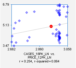
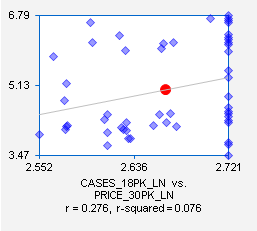
It is reasonable to expect that there will also be substitution effects,
i.e. “cross-price elasticities.” Consumers ought to buy relatively more
[fewer] 18-packs when the price of another carton size is raised [lowered]. Indeed, the correlations and
scatterplots for sales of 18-packs vs. prices of 12-packs and 30-packs (taken
from the original scatterplot matrix) suggest that there are such effects:
To test this hypothesis, let’s add these two variables to the
previous model. Here is the model
summary report produced by RegressIt:
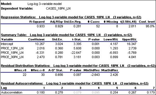
The
coefficients of the two additional variables are significantly different from
zero, and most importantly there has been a significant reduction in the
standard error of the regression, from 0.356 to 0.281. Recall that errors measured in log units
can be roughly interpreted as
percentages, if they are on the order of 0.2 or less. These numbers are a bit too large for
that approximation to fit very well, but still, very roughly speaking, the standard deviation of the errors in
percentage terms has been reduced from around 36% to around 28%, which is a
meaningful improvement. (Return to top of page.)
The
estimated coefficient of PRICE_18PK_PN (-6.331) is very close to its value in
the previous model, which is good:
it means the own-price effect is fairly robust to the manipulation of
the other prices. The estimated
coefficient of 0.2016 for PRICE_12PK_LN (its cross-price elasticity with
respect to sales of 18-packs) means roughly that a 1% increase [decrease] in
the price of 12-packs should be predicted to yield a 2% increase [decrease] in
sales of 18-packs, other things being equal. For 30-packs, whose coefficient is 2.47,
the effect is a little stronger.
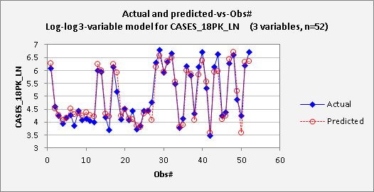
Now
for the plots. The
actual-and-predicted-vs-obs# plots appears to show a very nice fit:
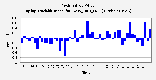
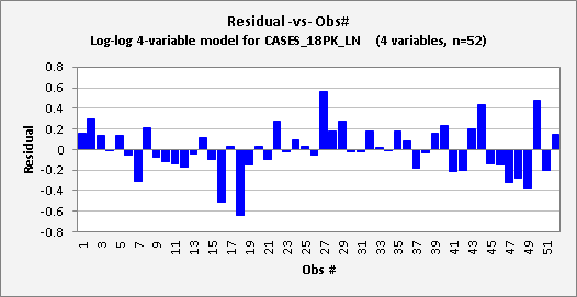
However,
the residual-vs-obs# plot indicates a bit of a problem: there
is a noticeable time pattern in the errors, namely an upward trend. (Errors in the first half of the year are
nearly all negative, while those in the second half are mostly positive.) This pattern is also reflected in the
residual autocorrelations, which are positive at lags 1 and 2: 0.18 and 0.278
respectively. These values are
actually not quite large enough in magnitude to be significant at the 0.05
level, although that is not a magical standard. (The critical value for this test is
roughly 2/SQRT(n), where n is the sample size, which is 0.28 in this case.) The appearance of the residual plot
rather than the values of the test statistics is the best diagnostic of the
time pattern here. Always look at
the pictures! (Return
to top of page.)
A linear trend in the errors of a
regression model can be addressed by including a time index variable (for example, the week-number variable in
this file) as another regressor. If
we do that here, we obtain the following 4-variable multiple regression model:
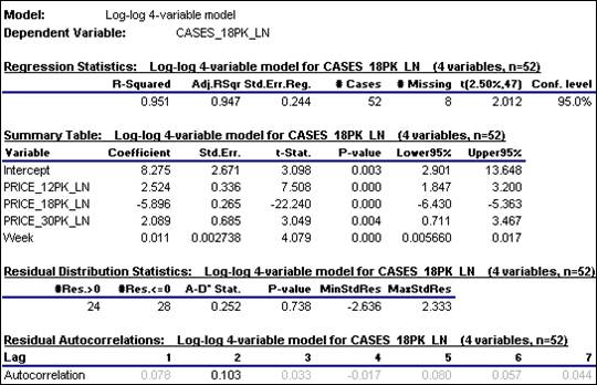
The
standard error of the regression has been further reduced by a meaningful
amount, from 0.281 to 0.244. The
coefficients of the original variables have wiggled around a bit, but are in the
same ballpark as before. The
coefficient of Week is significantly different from zero (t=4.079), and its
value of 0.011 appears to suggest that the average trend in sales of 18-packs
is about 1.1% per week. But
appearances can sometimes be deceiving:
in the context of a multiple
regression model, a trend variable adjusts for differences in trends among all
the variables, rather than measuring the trend in the dependent variable
alone. (Return
to top of page.)
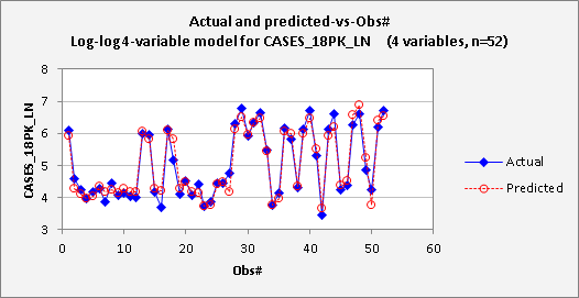
The updated
plots are shown below. The
residual-vs-obs# plot now does not show any systematic time pattern, and the
autocorrelations that were previously seen in the errors have essentially
vanished.
Overall,
this appears to be a good model, and it has a lot to say about how sales of
18-packs are affected by price. The
additional take-aways from this step of the analysis are that:
·
There is significant cross-price elasticity in the data for
sales of 18-packs vs. prices of 12-packs and 30-packs.
·
The trend in sales of 18-packs is not entirely explained by
trends in price
·
This exercise has illustrated the construction of a linear
regression model by a series of logical steps, beginning with descriptive
analysis and proceeding through the fitting of a sequence of models that are
motivated by economic theory and by interpretation of patterns seen in the
statistical and graphical output.
This
is not quite the end of the story:
some final comments and another picture are given below.
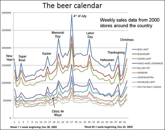
Postscript: this is real data, and one thing that is
a bit curious about it is that there is no evidence of seasonality. In general, beer sales in the U.S.
exhibit very significant seasonality, being higher in the hotter months and
having large spikes in certain holiday weeks. Here’s a picture of total weekly
sales of the top-selling brands at a much larger sample of stores: