Notes
on linear regression analysis (pdf)
Introduction to linear regression analysis
Mathematics
of simple regression
Regression examples
·
Beer sales vs. price, part 1: descriptive
analysis
·
Beer sales vs. price, part 2: fitting a simple
model
·
Beer sales vs. price, part 3: transformations
of variables
·
Beer sales vs.
price, part 4: additional predictors
·
NC natural gas
consumption vs. temperature
·
More regression datasets
at regressit.com
What to look for in
regression output
What’s a good
value for R-squared?
What's the bottom line?
How to compare models
Testing the assumptions of linear regression
Additional notes on regression analysis
Stepwise and all-possible-regressions
Excel file with
simple regression formulas
Excel file with regression
formulas in matrix form
Notes on logistic regression (new!)
If you use
Excel in your work or in your teaching to any extent, you should check out the
latest release of RegressIt, a free Excel add-in for linear and logistic
regression. See it at regressit.com. The linear regression version runs on both PC's and Macs and
has a richer and easier-to-use interface and much better designed output than
other add-ins for statistical analysis. It may make a good complement if not a
substitute for whatever regression software you are currently using,
Excel-based or otherwise. RegressIt is an excellent tool for
interactive presentations, online teaching of regression, and development of
videos of examples of regression modeling. It includes extensive built-in
documentation and pop-up teaching notes as well as some novel features to
support systematic grading and auditing of student work on a large scale. There
is a separate logistic
regression version with
highly interactive tables and charts that runs on PC's. RegressIt also now
includes a two-way
interface with R that allows
you to run linear and logistic regression models in R without writing any code
whatsoever.
If you have
been using Excel's own Data Analysis add-in for regression (Analysis Toolpak),
this is the time to stop. It has not
changed since it was first introduced in 1993, and it was a poor design even
then. It's a toy (a clumsy one at that), not a tool for serious work. Visit
this page for a discussion: What's wrong with Excel's Analysis Toolpak for regression
A simple regression example: predicting baseball batting
averages
Background and data
description
Larger
data file with many more variables (2.5M)
Background and data description
Sports analytics
is a booming field. Owners, coaches, and fans are using statistical measures
and models of all kinds to study the performance of players and teams. A very simple example is provided
by the study of yearly data on batting averages for individual players in the
sport of baseball. (If you are not
familiar with the sport, stop here and watch this video which explains
it all. Another very highly
recommended reference is this
movie.) The sample used here
contains 588 rows of data for a select group of players during the years
1960-2004, and it was obtained from the Lahman Baseball
Database. The Excel file with
the data and analysis can be found here.
The objective of this exercise will be to
predict a player’s batting average in a given year from his batting
average in the previous year and/or his cumulative batting average over all
previous years for which data is available. A much larger file with 4535 rows and 82
columns--more players and more statistical measures of performance--is also
included among the links above, in case you would like to do more analysis of
your own.
A
player’s batting average is the ratio of his number of hits to his number
of opportunities-to-hit (so-called “at-bats”). There are 162 games in the season,
and a regular position player (a non-pitcher who is a starter at his position)
typically has 4 or 5 at-bats per game and accumulates 600 or more in a season
if he does not miss many games due to injuries or being benched or suspended. Most players have batting averages
somewhere between 0.250 and 0.300.
Because a player’s batting average in a given year of his career
is an average of a very large number of (almost) statistically independent
random variables, it might be expected to be normally distributed around its
hypothetical true value that is determined by his innate hitting ability. Also, it is reasonable to expect that
these hypothetical true values are themselves approximately normally
distributed in the population and that they are to some extent
“inherited” from one year of a player’s career to the next
(like inheritability of size in Galton’s sweet
peas). Hence
we should not be surprised to find that the empirical distribution of batting
averages of all players across all years is very close to a normal distribution
and that a player’s performance in a given year is positively correlated
with his batting average in prior years and hence predictable by linear
regression. It is not actually
necessary for individual variables in a regression model to be normally
distributed—only the prediction errors need to be normally
distributed—but the case in which all the variables are normally distributed is the best-case scenario and yields the
prettiest pictures.
(The same type of analysis could be done with respect to statistical
measures of performance in other sports—say, scoring averages or free-throw
percentages in basketball—and qualitatively similar results would be
obtained. Regression-to-the-mean is
found everywhere.)
Each row in
the data file contains statistics for a single player for a single year in which the player had at least 400 at-bats
and also at least 400 at-bats in the previous year. The latter constraint was imposed to
ensure that only regular players (the best on their teams at their respective
positions) were included and also so that the sample size of at-bats for each
player was large. The statistics
for the analysis consist of batting average, batting average lagged by one
year, and cumulative batting average lagged by one year. The first few rows look like this:
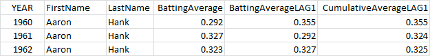
The term
“lagged” means “lagging behind” by a specified number
of periods, i.e., an observation of the same variable in an earlier
period. For example, Hank
Aaron’s value of 0.292 for BattingAverageLAG1 in 1961 is by definition
the same as the value of BattingAverage for him in 1960. In general in this file,
BattingAverageLAG1 in a given row is equal to BattingAverage in the previous
row if the previous row corresponds to
the previous year for the same player. (Return to
top of page.)
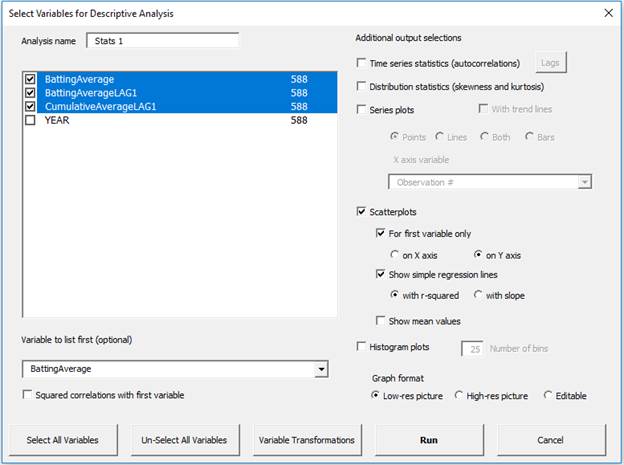
Let’s
start by looking at descriptive statistics of the 3 variables. Here are the specifications of the
analysis in RegressIt:
The results
are shown below. The mean value of
batting average is 0.277 (“two seventy seven” in baseball
language), and the means of the lagged averages and lagged cumulative averages
are only slightly different. The
correlation between batting average and lagged batting average (0.481) is a little
smaller than the correlation between batting average and lagged cumulative batting average (0.538),
i.e., the player’s batting average
in a given year is better predicted by his cumulative history of performance
than by his performance in the immediately preceding year.
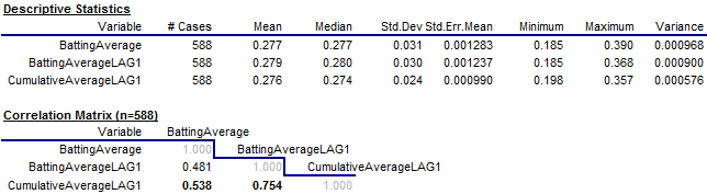
Note that
the correlation between lagged average and lagged cumulative average is 0.754.
which is much higher than the others.
This is an artifact of the way the set of years to include for a given
player was determined. In the
larger database from which this file was extracted, there are many players with
little or no history prior to their first 400-at-bat year, in which case their
lagged batting average and cumulative lagged batting average are very similar
if not identical in their first record in this file. This is true for Hank Aaron, as seen
above.
Now
let’s look at the scatterplots of batting average versus the two lagged
variables. They show almost perfect
bivariate normal distributions, as we might have expected for the reasons
mentioned above:
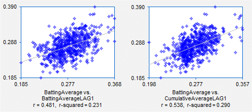
The
regression lines and squared correlations are included on the scatterplots (a
feature of RegressIt), so we have a good idea what to expect if simple
regression models are fitted.
(Return to top of page.)
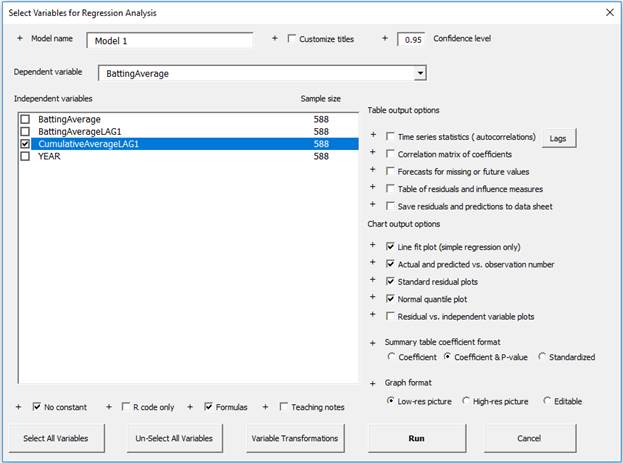
Because CumulativeAverageLAG1
is slightly more predictive than BattingAverageLAG1, let’s go ahead and
fit the model in which it is the independent variable from which BattingAverage
is predicted. Here are the model
specifications in RegressIt:
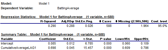
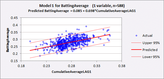
The summary
output and line fit plot are shown below. R-squared is 0.290, which we already knew, and adjusted R-squared is only slightly different (0.288), given the
large sample size. The standard error of the regression (which
is approximately the standard deviation of a forecast error) is 0.026, meaning
that a 95% confidence interval around a forecast is roughly the point forecast
plus-or-minus 0.052: quite a lot of
uncertainty!
The
estimated slope coefficient is
0.698, which means that a player whose prior cumulative average deviated from
the mean by the amount x is predicted to have a batting average that deviates
from the mean by about 0.7x in the current year, i.e., his batting average is
predicted to regress-to-the-mean by 30% relative to his prior cumulative
batting average. Recall that the way to think of a simple regression
model is that it predicts the dependent variable to deviate from its mean by an
amount equal to the slope coefficient times the deviation of the independent
variable from its mean. If you think of it that way, you
don’t need to pay attention to the intercept. The
precise value of the intercept is not of interest unless it is possible for the
independent variable to approach zero, which it can’t in this case,
otherwise the player would not be given hundreds of chances to bat in a given
year.
The standard error of the coefficient is
the (estimated) standard deviation of the error in estimating it, and the t-statistic is the coefficient estimate
divided by its own standard error, i.e., its “number of standard errors
from zero.” A t-statistic
whose value is 2 or larger in magnitude is generally considered to indicate
that the coefficient estimate is “significantly” different from
zero and hence that the variable has some genuine predictive value in the
context of the model. Here the
standard error of the slope coefficient (0.045) is very small in comparison to
the point estimate of the coefficient (0.698), so the corresponding t-statistic
is huge (greater than 15).
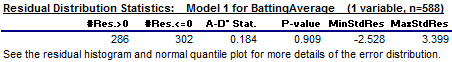
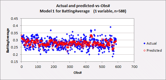
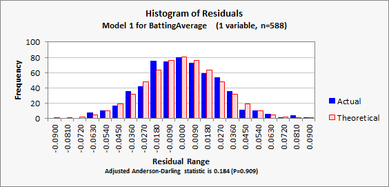
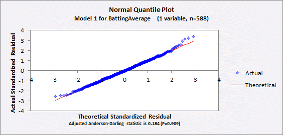
For the
record, the rest of the model’s output is shown below. The interpretation of such statistics
and plots is discussed in depth in other sections of these notes, but they look
very good here: there is no sign of any problem with the model’s
assumptions that the relationship between the variables is linear and that the
errors are independently and identically normally distributed. (Jump to
next section: multiple regression.) (Return to
top of page.)


From the
pairwise correlations, we know that CumulativeAverageLAG1 is better than BattingAverageLAG1 for
purposes of predicting BattingAverage via simple regression, but it could be
true that including both variables in
the model is better than including only one of them. To test this hypothesis, let’s add
BattingAverageLAG1 as a second regressor.
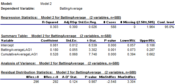
The summary output is shown below.
Both variables are highly significant, although R-squared rises only
from 0.290 to 0.303 and the standard error of the regression is unchanged (to 3
digits of precision). The
estimated coefficients of BattingAverageLAG1 and CumulativeAverageLAG1 are
0.180 and 0.528, respectively, and both are significantly different from zero
as indicated their very large t-statistics (greater than3.3 and 7.7,
respectively)
On the basis
of the error stats alone, it would be hard to argue that the increase in model
complexity is worth it, except that the pattern of the coefficients is in line
with intuition. The coefficient of
lagged cumulative average was 0.698 in the first model. In the second model, both coefficients are
positive and their sum is 0.708, which is essentially the same as the
coefficient in the first model.
This means that the second model
merely reallocates some of the weight on prior performance to place a little
more on the most recent year’s average. So, even though the second model does
not noticeably reduce the standard error of the regression with the addition of
another variable, it can still be defended on the basis that it makes sense to
place a little more weight on the most recently observed batting average value,
rather than use a somewhat arbitrary equally weighted average of all available
past data. This example illustrates
that in fitting a model, there is more to be done than to look at error statistics
and significance tests. Interpreting
the values and meaning of the coefficients is also a part of the analysis. (Return
to top of page.)
Go on to example #2: predicting weekly beer sales