
Notes on linear
regression analysis (pdf file)
Introduction
to linear regression analysis
Mathematics
of simple regression
Regression examples
·
Beer sales vs. price, part 1: descriptive
analysis
·
Beer sales vs. price, part 2: fitting a simple
model
·
Beer sales vs. price, part 3: transformations
of variables
·
Beer sales vs.
price, part 4: additional predictors
·
NC natural gas
consumption vs. temperature
·
More regression datasets
at regressit.com
What to look for in
regression output
What’s a good
value for R-squared?
What's the bottom line? How to compare models
Testing the assumptions of
linear regression
Additional notes on regression analysis
Stepwise and all-possible-regressions
Excel file with
simple regression formulas
Excel file with regression
formulas in matrix form
Notes on logistic regression (new!)
If you use Excel
in your work or in your teaching to any extent, you should check out the latest
release of RegressIt, a free Excel add-in for linear and logistic regression.
See it at regressit.com. The linear regression version runs on both PC's and Macs and
has a richer and easier-to-use interface and much better designed output than
other add-ins for statistical analysis. It may make a good complement if not a
substitute for whatever regression software you are currently using,
Excel-based or otherwise. RegressIt is an excellent tool for
interactive presentations, online teaching of regression, and development of
videos of examples of regression modeling. It includes extensive built-in
documentation and pop-up teaching notes as well as some novel features to
support systematic grading and auditing of student work on a large scale. There
is a separate logistic
regression version with
highly interactive tables and charts that runs on PC's. RegressIt also now
includes a two-way
interface with R that allows
you to run linear and logistic regression models in R without writing any code
whatsoever.
If you have
been using Excel's own Data Analysis add-in for regression (Analysis Toolpak),
this is the time to stop. It has not
changed since it was first introduced in 1993, and it was a poor design even
then. It's a toy (a clumsy one at that), not a tool for serious work. Visit
this page for a discussion: What's wrong with Excel's Analysis Toolpak for regression
Additional notes on
linear regression analysis
To include or not to include the CONSTANT?
Interpreting STANDARD ERRORS, "t" STATISTICS, and
SIGNIFICANCE LEVELS of coefficients
Interpreting the F-RATIO
Interpreting
measures of multicollinearity: CORRELATIONS AMONG COEFFICIENT ESTIMATES and VARIANCE INFLATION FACTORS
Interpreting CONFIDENCE INTERVALS
TYPES of confidence intervals
Dealing with OUTLIERS
Caution: MISSING
VALUES may cause variations in SAMPLE SIZE
MULTIPLICATIVE regression models and the LOGARITHM
transformation
To
include or not to include the CONSTANT?
Most
multiple regression models include a constant term (i.e., an
"intercept"), since this ensures that the model will be unbiased--i.e., the mean of the
residuals will be exactly zero. (The coefficients in a regression model
are estimated by least squares--i.e., minimizing the mean squared error. Now, the
mean squared error is equal to the variance of the errors plus the square of
their mean: this is a mathematical identity. Changing the value of the
constant in the model changes the mean of the errors but doesn't affect the
variance. Hence, if the sum of squared errors is to be minimized, the constant must
be chosen such that the mean of the errors is zero.) In a simple regression
model, the constant represents the Y-intercept of the regression line, in
unstandardized form. In a multiple regression model, the constant represents
the value that would be predicted for the dependent variable if all the
independent variables were simultaneously equal to zero--a situation which may
not physically or economically meaningful. If
you are not particularly interested in what would happen if all the independent
variables were simultaneously zero, then you normally leave the constant in the model regardless of its statistical
significance. In addition to ensuring that the in-sample errors are unbiased, the presence of the
constant allows the regression line to "seek its own level" and
provide the best fit to data which may only be locally linear.
However, in
rare cases you may wish to exclude
the constant from the model. This is a model-fitting option in the regression
procedure in any software package, and it is sometimes referred to as regression through the origin, or RTO for short. Usually, this will be
done only if (i) it is possible to imagine the independent variables all
assuming the value zero simultaneously, and you feel that in this case it
should logically follow that the dependent variable will also be equal to zero;
or else (ii) the constant is redundant with the set of independent variables
you wish to use. An example of case (i) would be a model in which all
variables--dependent and independent--represented first differences
of other time series. If you are regressing the first difference of Y on the
first difference of X, you are directly predicting changes in Y as a linear function of changes
in X, without reference to the current
levels of the variables. In this case it might be reasonable (although
not required) to assume that Y
should be unchanged, on the average, whenever X is unchanged--i.e., that Y should not have an upward or downward trend in the
absence of any change in the level of X.
An example of case (ii) would be a situation in which you wish to use a full
set of seasonal indicator variables--e.g., you are
using quarterly data, and you wish to include variables Q1, Q2, Q3, and Q4
representing additive seasonal effects. Thus, Q1 might look like 1 0 0 0 1 0 0
0 ..., Q2 would look like 0 1 0 0 0 1 0 0 ..., and so on. You could not use all
four of these and a constant in the same model, since Q1+Q2+Q3+Q4 = 1 1
1 1 1 1 1 1 . . . . , which is the same as a constant
term. I.e., the five variables Q1, Q2, Q3, Q4, and CONSTANT are not linearly
independent: any one of them can be expressed as a linear combination of
the other four. A technical prerequisite for fitting a linear regression model
is that the independent variables must be linearly independent;
otherwise the least-squares coefficients cannot be determined uniquely,
and we say the regression "fails."
A word of
warning: R-squared and the F
statistic do not have the same meaning in an RTO model as they do in an
ordinary regression model, and they are not calculated in the same way by all
software. See page 77 of this
article for the formulas and some caveats about RTO in general. You should not try to compare R-squared
between models that do and do not include a constant term, although it is OK to
compare the standard error of the regression.
Note that
the term "independent" is used in (at least) three different ways in
regression jargon: any single variable may be called an independent
variable if it is being used as a predictor, rather than as the predictee.
A group of variables is linearly independent if no one of them
can be expressed exactly as a linear combination of the others. A pair
of variables is said to be statistically independent if they are not
only linearly independent but also utterly uninformative with respect to each
other. In a regression model, you want your dependent variable to be statistically
dependent on the independent variables, which must be linearly
(but not necessarily statistically) independent among themselves. Got
it? (Return to top
of page.)
Interpreting
STANDARD ERRORS, t-STATISTICS, AND SIGNIFICANCE LEVELS OF COEFFICIENTS
Your
regression output not only gives point estimates of the coefficients of
the variables in the regression equation, it also gives information about the precision
of these estimates. Under the assumption that your regression model is
correct--i.e., that the dependent variable really is a linear function of the
independent variables, with independent and identically normally distributed
errors--the coefficient estimates are expected to be unbiased and their errors
are normally distributed. The standard errors of the coefficients are
the (estimated) standard deviations of the errors in estimating them.
In general, the standard error of the coefficient for variable X is equal to the standard error of
the regression times a factor that depends only on the values of X and the other independent variables
(not on Y), and which is
roughly inversely proportional to the standard deviation of X. Now, the standard error of the
regression may be considered to measure the overall amount of "noise"
in the data, whereas the standard deviation of X measures the strength
of the "signal" in X.
Hence, you can think of the standard error of the estimated coefficient of X
as the reciprocal of the signal-to-noise ratio for observing the effect of X on Y. The larger the standard error of the coefficient
estimate, the worse the signal-to-noise ratio--i.e., the less precise
the measurement of the coefficient.
The t-statistics for the independent
variables are equal to their coefficient estimates divided by their respective
standard errors.
In theory, the t-statistic of any one variable may be used to test the
hypothesis that the true value of the coefficient is zero (which
is to say, the variable should not be included in the model). If the
regression model is correct (i.e., satisfies the "four
assumptions"), then the estimated values of the coefficients should be
normally distributed around the true values. In particular, if the true value
of a coefficient is zero, then its estimated coefficient should be normally
distributed with mean zero. If the standard deviation of this normal
distribution were exactly known, then the coefficient estimate divided by the
(known) standard deviation would have a standard normal distribution,
with a mean of 0 and a standard deviation of 1. But the standard deviation is not
exactly known; instead, we have only an estimate of it, namely the
standard error of the coefficient estimate. Now, the coefficient estimate
divided by its standard error does not have the standard normal distribution,
but instead something closely related: the "Student's t" distribution
with n - p degrees of freedom, where n is the number of
observations fitted and p is the number of coefficients estimated,
including the constant. The t distribution resembles the standard normal
distribution, but has somewhat fatter tails--i.e., relatively more extreme
values. However, the difference between the t and the standard normal is
negligible if the number of degrees of freedom is more than about 30.
In a
standard normal distribution, only 5% of the values fall outside the range
plus-or-minus 2. Hence, as a rough rule of thumb, a t-statistic larger than 2
in absolute value would have a 5% or smaller probability of occurring by chance
if the true coefficient were zero. Most stat packages will compute for you the exact
probability of exceeding the observed t-value by chance if the true coefficient
were zero. This is labeled as the "P-value" or "significance
level" in the table of model coefficients. A low value for this probability
indicates that the coefficient is significantly different from zero,
i.e., it seems to contribute something to the model.
Usually you
are on the lookout for variables that could be removed without seriously
affecting the standard error of the regression. A low t-statistic (or
equivalently, a moderate-to-large exceedance probability) for a variable
suggests that the standard error of the regression would not be adversely
affected by its removal. The commonest rule-of-thumb in this regard is to remove
the least important variable if its t-statistic is less than 2 in
absolute value, and/or the exceedance probability is greater than .05.
Of course, the proof of the pudding is still in the eating: if you remove a
variable with a low t-statistic and this leads to an undesirable increase in
the standard error or the regression (or deterioration of some other
statistics, such as residual autocorrelations), then you should probably put it
back in.
Generally you should only add
or remove variables one at a time, in a stepwise fashion, since when one
variable is added or removed, the other variables may increase or decrease in
significance. For example, if X1
is the least significant variable in the original regression, but X2 is almost equally
insignificant, then you should try removing X1 first and see what happens to the estimated
coefficient of X2:
the latter may remain insignificant after X1 is removed, in which case you might try removing X2 as well, or it may rise
in significance (with a very different estimated value), in which case you may
wish to leave it in.
Note: the
t-statistic is usually not used as a basis for deciding whether or not
to include the constant term. Usually the decision to include or exclude
the constant is based on a priori reasoning, as noted above. If it is
included, it may not have direct economic significance, and you generally don't
scrutinize its t-statistic too closely.
Return to top of page
The F-ratio
and its exceedance probability provide a test of the significance of all the independent variables (other
than the constant term) taken together. The variance of the dependent
variable may be considered to initially have n-1 degrees of freedom,
since n observations are initially available (each including an error
component that is "free" from all the others in the sense of
statistical independence); but one degree of freedom is used up in computing
the sample mean around which to measure the variance--i.e., in estimating the constant
term alone. As noted above, the effect of fitting a regression model with p
coefficients including the constant is to decompose this variance into an
"explained" part and an "unexplained" part. The explained
part may be considered to have used up p-1 degrees of freedom
(since this is the number of coefficients estimated besides the
constant), and the unexplained part has the remaining unused n - p
degrees of freedom.
The F-ratio
is the ratio of the explained-variance-per-degree-of-freedom-used to the
unexplained-variance-per-degree-of-freedom-unused, i.e.:
F =
((Explained variance)/(p-1) )/((Unexplained
variance)/(n - p))
Now, a set
of n observations could in principle be perfectly fitted by a
model with a constant and any n - 1 linearly independent other
variables--i.e., n total variables--even if the independent variables
had no predictive power in a statistical sense. This suggests that any irrelevant
variable added to the model will, on the average, account for a fraction 1/(n-1)
of the original variance. Thus, if the true values of the coefficients are all
equal to zero (i.e., if all the independent variables are in fact
irrelevant), then each coefficient estimated might be expected to merely soak
up a fraction 1/(n - 1) of the original
variance. In this case, the numerator and the denominator of the F-ratio should
both have approximately the same expected value; i.e., the F-ratio should be
roughly equal to 1. On the other hand, if the coefficients are really not
all zero, then they should soak up more than their share of the variance, in
which case the F-ratio should be significantly larger than 1. Standard regression output includes the
F-ratio and also its exceedance probability--i.e., the probability of getting
as large or larger a value merely by chance if the true coefficients were all
zero. (In Statgraphics this is shown in the ANOVA table obtained by selecting
"ANOVA" from the tabular options menu that appears after fitting the
model. The ANOVA table is also
hidden by default in RegressIt output but can be displayed by clicking the
"+" symbol next to its title.) As with the exceedance probabilities
for the t-statistics, smaller is better. A low exceedance probability
(say, less than .05) for the F-ratio suggests that at least some of the
variables are significant.
In a simple
regression model, the F-ratio is simply the
square of the t-statistic of the (single) independent variable, and the
exceedance probability for F is the same as that for t. In a multiple
regression model, the exceedance probability for F will generally be smaller
than the lowest exceedance probability of the t-statistics of the independent
variables (other than the constant). Hence, if at least one variable is
known to be significant in the model, as judged by its t-statistic, then there
is really no need to look at the F-ratio. The F-ratio is useful primarily in
cases where each of the independent variables is only marginally significant by
itself but there are a priori grounds for believing that they are significant
when taken as a group, in the context of a model where there is a logical way
to group them. For example, the
independent variables might be dummy variables for treatment levels in a
designed experiment, and the question might be whether there is evidence for an
overall effect, even if its fine detail cannot quantified
precisely with the given sample size.
(Return to top of page.)
Interpreting measures of multicollinearity:
CORRELATIONS AMONG COEFFICIENT ESTIMATES and
VARIANCE INFLATION FACTORS
It often
happens that there are several available independent variables that are
plausibly linearly related to the dependent variable but also strongly linearly
related to each other. That is to
say, their information value is not really independent with respect to
prediction of the dependent variable in the context of a linear model. (Such a situation is often
observed, for example, when the independent variables are a collection of
economic indicators that are computed from some of the same underlying data via
weighted averages.) This condition
is referred to as multicollinearity. In the most extreme cases of
multicollinearity--e.g., when one of the independent variables is an exact
linear combination of some of the others--the regression calculation will fail,
and you will need to look closely at the definitions of your variables to
determine which ones are the culprits.
Sometimes one variable is merely a rescaled copy of another variable or
a sum or difference of other variables, and sometimes a set of dummy variables
adds up to a constant variable
The correlation
matrix of the estimated coefficients (if your software includes it)
is one diagnostic tool for detecting relative degrees of multicollinearity. It
shows the extent to which particular pairs
of variables provide independent information for purposes of predicting the dependent variable, given the
presence of other variables in the model. Extremely high values here (say,
much above 0.9 in absolute value) suggest that some pairs of variables are not
providing independent information.
In this case, either (i) both variables are providing the same
information--i.e., they are redundant; or (ii) there is some linear
function of the two variables (e.g., their sum or difference) that
summarizes the information they carry.
In case
(i)--i.e., redundancy--the estimated coefficients of the two variables are
often large in magnitude, with standard errors that are also large, and they
are not economically meaningful.
When this happens, it is usually desirable to try removing one of them,
usually the one whose coefficient has the higher P-value. In case (ii), it may be possible to
replace the two variables by the appropriate linear function (e.g., their sum
or difference) if you can identify it, but this is not strictly
necessary. This situation often arises when two or more different lags of
the same variable are used as independent variables in a time series
regression model. (Coefficient
estimates for different lags of the dependent variable are often highly
correlated, but this may or may not be a problem unless the pattern of their
coefficients is such that there is a “unit
root” in the resulting equation.
See the mathematics-of-ARIMA-models
notes for more discussion of unit roots.)
Many
statistical analysis programs report variance
inflation factors (VIF’s), which are another measure of
multicollinearity, in addition to or instead of the correlation matrix of
coefficient estimates. The VIF of an independent variable is the
value of 1 divided by 1-minus-R-squared in a regression of itself on the other
independent variables. The rule
of thumb here is that a VIF larger than
10 is an indicator of potentially significant multicollinearity between
that variable and one or more others.
(Note that a VIF larger than 10 means that the regression of that
independent variable on the others has an R-squared of greater than 90%.) If this is observed, it means that the
variable in question does not contain much independent information in the
presence of all the other variables,
taken as a group. When this
happens, it often happens for many variables at once, and it may take some
trial and error to figure out which one(s) ought to be removed. However, like most other diagnostic
tests, the VIF-greater-than-10 test is not a hard-and-fast rule, just an
arbitrary threshold that indicates the possibility
of a problem. In this case it
indicates a possibility that the model could be simplified, perhaps by deleting
variables or perhaps by redefining them in a way that better separates their
contributions.
Interpreting
CONFIDENCE INTERVALS
Suppose that
you fit a regression model to a certain time series--say, some sales data--and
the fitted model predicts that sales in the next period will be $83.421M. Does
this mean you should expect sales to be exactly $83.421M? Of course not.
This is merely what we would call a "point estimate" or "point
prediction." It should really be considered as an average taken
over some range of likely values. For a point estimate to be really useful, it
should be accompanied by information concerning its degree of precision--i.e.,
the width of the range of likely values. We would like to be able to state how confident
we are that actual sales will fall within a given distance--say, $5M or
$10M--of the predicted value of $83.421M.
In
"classical" statistical methods such as linear regression,
information about the precision of point estimates is usually expressed in the
form of confidence intervals. For example, the regression model above
might yield the additional information that "the 95% confidence interval
for next period's sales is $75.910M to $90.932M." Does this mean that,
based on all the available data, we should conclude that there is a 95% probability
of next period's sales falling in the interval from $75.910M to $90.932M? That
is, should we consider it a "19-to-1 long shot" that sales would fall
outside this interval, for purposes of betting? The answer to this is:
- No,
strictly speaking, a confidence interval is not a probability interval for
purposes of betting.
Rather, a 95% confidence interval is an interval
calculated by a formula having the property that, in the long run, it will cover the true value 95% of the time in
situations in which the correct model
has been fitted. In other
words, if everybody all over the world used this formula on correct models
fitted to his or her data, year in and year out, then you would expect an
overall average "hit rate" of 95%. Alas, you never know for sure
whether you have identified the
correct model for your data, although
residual diagnostics help you rule out obviously incorrect ones. So, on your data today there
is no guarantee that 95% of the computed confidence intervals will cover the
true values, nor that a single confidence interval has, based on the available
data, a 95% chance of covering the true value. This is not to say that a
confidence interval cannot be meaningfully interpreted, but merely that it
shouldn't be taken too literally in any single case, especially if there is any
evidence that some of the model assumptions are not correct.
In fitting a
model to a given data set, you are often simultaneously estimating many things:
e.g., coefficients of different variables, predictions for different future
observations, etc. Thus, a model for a given data set may yield many
different sets of confidence intervals. You may wonder whether it is valid
to take the long-run view here: e.g., if I calculate 95% confidence intervals
for "enough different things" from the same data, can I expect about
95% of them to cover the true values? The answer to this is:
- No,
multiple confidence intervals calculated from a single model fitted to a
single data set are not independent with respect to their chances of
covering the true values.
This is
another issue that depends on the correctness of the model and the
representativeness of the data set, particularly in the case of time series
data. If the model is not correct
or there are unusual patterns in the data, then if the confidence interval for
one period's forecast fails to cover the true value, it is relatively more
likely that the confidence interval for a neighboring period's forecast will
also fail to cover the true value, because the model may have
a tendency to make the same error for several periods in a row.
Ideally, you
would like your confidence intervals to be as narrow as possible: more
precision is preferred to less. Does this mean that, when comparing alternative
forecasting models for the same time series, you should always pick the one
that yields the narrowest confidence intervals around forecasts? That is,
should narrow confidence intervals for forecasts be considered as a sign of a
"good fit?" The answer, alas, is:
- No,
the best model does not necessarily yield the narrowest confidence
intervals around forecasts.
If the
model's assumptions are correct, the confidence intervals it yields will be realistic
guides to the precision with which future observations can be predicted. If the
assumptions are not correct, it may yield confidence intervals that are all
unrealistically wide or all unrealistically narrow. That is to say, a
bad model does not necessarily know it is a bad model, and warn you by
giving extra-wide confidence intervals. (This is especially true of trend-line
models, which often yield overoptimistically narrow confidence intervals for
forecasts.) You need to judge whether the model is good or bad by looking at
the rest of the output.
Notwithstanding
these caveats, confidence intervals are indispensable, since they are usually
the only estimates of the degree of precision in your coefficient
estimates and forecasts that are provided by most stat packages. And, if (i)
your data set is sufficiently large, and your model passes the diagnostic tests
concerning the "4
assumptions of regression analysis," and (ii) you don't have strong
prior feelings about what the coefficients of the variables in the model should
be, then you can treat a 95% confidence interval as an approximate
95% probability interval. (In the long run.) (Return to top of page.)
In
regression forecasting, you may be concerned with point estimates and
confidence intervals for some or all of the following:
- The
coefficients of the independent variables
- The mean of the dependent variable
(i.e., the true location of the
regression line) for given values of the independent variables
- The
prediction of the dependent variable for given values of the
independent variables
In all
cases, there is a simple relationship between the point estimate and its
surrounding confidence interval:
(Confidence
Interval) = (Point Estimate) + (Critical t-value) x (Standard Deviation
or Standard Error)
For a 95%
confidence interval, the "critical t value" is the value that
is exceeded with probability 0.025 (one-tailed) in a t distribution with
n-p degrees of freedom, where p is the number of coefficients in the
model--including the constant term if any. (In general, for a 100*(1-x) percent
confidence interval, you would use the t value exceeded with probability
x/2.) If the number of degrees of freedom is large--say, more than 30--the t
distribution closely resembles the standard normal distribution, and the
relevant critical t value for a 95% confidence interval is approximately
equal to 2. (More precisely, it is 1.96.) In this case, therefore, the 95%
confidence interval is roughly equal to the point estimate "plus or minus two standard
deviations." Here is a selection of critical t
values to use for different confidence intervals and different numbers of
degrees of freedom, taken from a standard table of the t distribution:
Degrees of t-value
for confidence interval
Freedom (n-p) 50% 80% 90% 95%
-------------- ------ ------ ------ ------
10
0.700 1.372 1.812 2.228
20
0.687 1.325 1.725 2.086
30
0.683 1.310 1.697 2.042
60
0.679 1.296 1.671 2.000
Infinite
0.674 1.282 1.645 1.960
A t-distribution
with "infinite" degrees of freedom is a standard normal distribution.
The "standard
error” or “standard deviation" in the above equation depends
on the nature of the thing for which you are computing the confidence interval.
For the confidence interval around a coefficient estimate, this is
simply the "standard error of the coefficient estimate" that appears
beside the point estimate in the coefficient table. (Recall that this is
proportional to the standard error of the regression, and inversely proportional
to the standard deviation of the independent variable.)
For a confidence
interval for the mean (i.e., the true height of the regression line), the relevant standard deviation
is referred to as the "standard deviation of the mean" at that point.
This quantity depends on the following factors:
- The
standard error of the regression
- the
standard errors of all the coefficient estimates
- the
correlation matrix of the coefficient estimates
- the
values of the independent variables at that point
Other things being
equal, the standard deviation of the mean--and hence the width of the
confidence interval around the regression line--increases with the
standard errors of the coefficient estimates, increases with the
distances of the independent variables from their respective means, and decreases
with the degree of correlation between the coefficient estimates. However, in a model characterized
by "multicollinearity", the standard errors of the coefficients and
For a confidence
interval around a prediction based on the regression line at some point,
the relevant standard deviation is called the "standard deviation of the
prediction." It reflects the error in the estimated height of the
regression line plus the true error, or "noise," that is
hypothesized in the basic model:
DATA = SIGNAL + NOISE
In this case, the
regression line represents your best estimate of the true signal, and the
standard error of the regression is your best estimate of the standard
deviation of the true noise. Now (trust me), for essentially the same reason
that the fitted values are uncorrelated with the residuals, it is also true
that the errors in estimating the height of the regression line are
uncorrelated with the true errors. Therefore, the variances of these two
components of error in each prediction are additive. Since variances are
the squares of standard deviations, this means:
(Standard deviation
of prediction)^2 = (Standard deviation of mean)^2 +
(Standard error of regression)^2
Note that, whereas
the standard error of the regression is a fixed number, the standard deviations
of the predictions and the standard deviations of the means will usually vary
from point to point in time, since they depend on the values of the independent
variables. However, the standard error of the regression is typically much
larger than the standard errors of the means at most points, hence the standard
deviations of the predictions will often not vary by much from point to
point, and will be only slightly larger than the standard error of the
regression.
It is possible to
compute confidence intervals for either means or predictions around the fitted
values and/or around any true forecasts which may have been
generated. Statgraphics and RegressIt will automatically generate forecasts rather
than fitted values wherever the dependent variable is "missing" but
the independent variables are not. Confidence intervals for the forecasts are
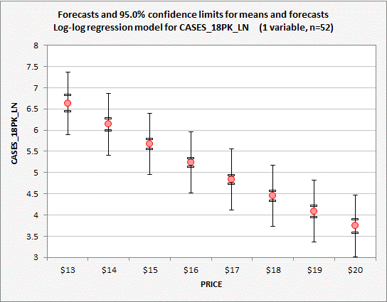
also reported. Here is an example
of a plot of forecasts with confidence limits for means and forecasts produced
by RegressIt for the regression
model fitted to the natural log of cases of 18-packs sold. If you look closely, you will see that
the confidence intervals for means (represented by the inner set of bars around
the point forecasts) are noticeably wider for extremely high or low values of
price, while the confidence intervals for forecasts are not.
One of the underlying
assumptions of linear regression analysis is that the distribution of the
errors is approximately normal with a mean of zero. A normal distribution has
the property that about 68% of the values will fall within 1 standard deviation
from the mean (plus-or-minus), 95% will fall within 2 standard deviations, and
99.7% will fall within 3 standard deviations. Hence, a value more than 3
standard deviations from the mean will occur only rarely: less than one out of
300 observations on the average. Now, the residuals from fitting a model may be
considered as estimates of the true errors that occurred at different points in
time, and the standard error of the regression is the estimated standard
deviation of their distribution. Hence, if the normality assumption is
satisfied, you should rarely encounter a residual whose absolute value is
greater than 3 times the standard error of the regression. An observation whose
residual is much greater than 3 times the standard error of the regression is
therefore usually called an "outlier." In the "Reports"
option in the Statgraphics regression procedure, residuals greater than 3 times
the standard error of the regression are marked with an asterisk (*). In the residual table in RegressIt,
residuals with absolute values larger than 2.5 times the standard error of the
regression are highlighted in boldface and those absolute values are larger
than 3.5 times the standard error of the regression are further highlighted in
red font. Outliers are also readily
spotted on time-plots and normal probability plots of the residuals.
If your data set
contains hundreds of observations, an outlier or two may not be cause for
alarm. But outliers can spell trouble for models fitted to small data sets:
since the sum of squares of the residuals is the basis for estimating
parameters and calculating error statistics and confidence intervals, one or
two bad outliers in a small data set can badly skew the results. When outliers
are found, two questions should be asked: (i) are they merely
"flukes" of some kind (e.g., data entry errors, or the result of
exceptional conditions that are not expected to recur), or do they represent
real and potentially repeatable events whose effects ought to be measured
(either by keeping them in the model or investigating separately); and (ii) how
much have the coefficients, error statistics, and predictions, etc., been
affected?
An outlier may or may
not have a dramatic effect on a model, depending on the amount of
"leverage" that it has. Its leverage depends on the values of the
independent variables at the point where it occurred: if the independent
variables were all relatively close to their mean values, then the
outlier has little leverage and will mainly affect the value of the
estimated CONSTANT term and the standard error of the regression. However, if
one or more of the independent variable had relatively extreme values at
that point, the outlier may have a large influence on the estimates of
the corresponding coefficients: e.g., it may cause an otherwise insignificant
variable to appear significant, or vice versa.
The best way to
determine how much leverage an outlier (or group of outliers) has, is to exclude
it from fitting the model, and compare the results with those originally
obtained. You can do this in Statgraphics by using the WEIGHTS option: e.g., if
outliers occur at observations 23 and 59, and you have already created a
time-index variable called INDEX, you could type:
INDEX <> 23
& INDEX <> 59
in the WEIGHTS field
on the input panel, and then re-fit the model. In RegressIt you can just delete the
values of the dependent variable in those rows. (Be sure to keep a copy of them, though! In this sort of exercise, it is best to
copy all the values of the dependent variable to a new column, assign it a new
variable name, then delete the desired values in the new column and use it as
the new dependent variable.)
Forecasts will automatically be generated for the excluded or missing values
of the dependent variable in either program. The discrepancies between the
forecasts and the actual values, measured in terms of the corresponding
standard-deviations-of- predictions, provide a guide to how
"surprising" these observations really were.
An alternative
method, which is often used in stat packages lacking a WEIGHTS option, is to
"dummy out" the outliers: i.e., add a dummy variable for each
outlier to the set of independent variables. These observations will then
be fitted with zero error independently of everything else, and the same
coefficient estimates, predictions, and confidence intervals will be obtained
as if they had been excluded outright. (However, statistics such as
R-squared and MAE will be somewhat different, since they depend on the
sum-of-squares of the original observations as well as the sum of squared
residuals, and/or they fail to correct for the number of coefficients
estimated.) In Statgraphics, to dummy-out the observations at periods 23 and
59, you could add the two variables:
INDEX = 23
INDEX = 59
to the set of
independent variables on the model-definition panel. In RegressIt you could create these
variables by filling two new columns with 0’s and then entering 1’s
in rows 23 and 59 and assigning variable names to those columns. The estimated coefficients for the two
dummy variables would exactly equal the difference between the offending
observations and the predictions generated for them by the model.
If it turns out the
outlier (or group thereof) does have a significant effect on the model,
then you must ask whether there is justification for throwing it out. Go back
and look at your original data and see if you can think of any explanations for
outliers occurring where they did. Sometimes you will discover data entry
errors: e.g., "2138" might have been punched instead of
"3128." You may discover some other reason: e.g., a strike or stock
split occurred, a regulation or accounting method was changed, the company
treasurer ran off to Panama, etc. In this case, you must use your own judgment
as to whether to merely throw the observations out, or leave them in, or
perhaps alter the model to account for additional effects.
CAUTION: MISSING VALUES MAY CAUSE VARIATIONS IN
SAMPLE SIZE
When dealing with many variables, particularly ones that may have been
obtained from different sources, it is not uncommon for some of them to have
missing values, often at the beginning or end (due to different amounts of
history and/or the use of time transformations such as lagging and
differencing), but sometimes in the middle as well. This may create a situation in which the
size of the sample to which the model is fitted may vary from model to model,
sometimes by a lot, as different variables are added or removed. (In general the estimation procedure
will use all rows of data in which none of the currently selected variables has
missing values.) You should always
keep your eye on the sample size that is reported in your output, to make sure
there are no surprises. Small
differences in sample sizes are not necessarily a problem if the data set is
large, but you should be alert for situations in which relatively many rows of
data suddenly go missing when more variables are added to the model. If this does occur, then you may have to
choose between (a) not using the variables that have significant numbers of
missing values, or (b) deleting all rows of data in which any of the variables
have missing values, so that the sample will be the same for any model that is
fitted.
Another thing to be aware of in regard to missing values is that
automated model selection methods such as stepwise
regression base their calculations on a covariance matrix computed in
advance from rows of data where all
of the candidate variables have non-missing values, hence the variable selection process will
overlook the fact that different sample sizes are available for different
models. For this reason, the value
of R-squared that is reported for a given model in the stepwise regression
output may not be the same as you would get if you fitted that model by
itself. (Return
to top of page.)
MULTIPLICATIVE
REGRESSION MODELS AND THE LOGARITHM TRANSFORMATION
The basic linear
regression model assumes that the contributions of the different independent variables
to the prediction of the dependent variable are additive. For example,
if X1 and X2 are assumed to contribute additively to Y,
the prediction equation of the regression model is:
Ŷt = b0 +
b1X1t
+ b2X2t
Here, if X1
increases by one unit, other things being equal, then Y is expected to increase
by b1 units. That
is, the absolute change in Y is proportional to the absolute
change in X1, with the coefficient b1 representing the constant of proportionality.
Similarly, if X2 increases by 1 unit, other things equal, Y is
expected to increase by b2 units. And if both X1
and X2 increase by 1 unit, then Y is expected to change by b1 + b2 units.
That is, the total expected change in Y is determined by adding
the effects of the separate changes in X1 and X2.
In some situations,
though, it may be felt that the dependent variable is affected multiplicatively
by the independent variables. This means that on the margin (i.e., for small
variations) the expected percentage change in Y should be proportional
to the percentage change in X1, and similarly for X2. And further, if X1 and X2
both change, then on the margin the expected total percentage change in
Y should be the sum of the percentage changes that would have resulted
separately. (For large variations, the percentages would be compounded, not
added.) The appropriate model for this situation is the multiplicative regression model:
Ŷt = b0 (X1t ^ b1)(X2t
^ b2)
Here, Y is
proportional to the product of X1 and X2, each
raised to some power, whose value we can try to estimate from the data.
(I am using Excel notation here, in which “^” stands for
“raised to the power of.”)
The coefficients b1
and b2 are referred to as the elasticities of Y with
respect to X1 and X2, respectively. If either of them is
equal to 1, we say that the response of Y to that variable has unitary
elasticity--i.e., the expected marginal percentage change in Y is exactly the
same as the percentage change in the independent variable. If the coefficient
is less than 1, the response is said to be inelastic--i.e., the
expected percentage change in Y will be somewhat less than the
percentage change in the independent variable.
The multiplicative model,
in its raw form above, cannot be fitted using linear regression techniques.
However, it can be converted into an equivalent linear model via the logarithm
transformation. The natural logarithm function (LOG in Statgraphics, LN in
Excel and RegressIt and most other mathematical software), has the property
that it converts products into sums: LOG(X1X2)
= LOG(X1)+LOG(X2), for any positive X1 and X2. Also, it converts powers into
multipliers: LOG(X1^b1)
= b1(LOG(X1)). Using these rules,
we can apply the logarithm transformation to both sides of the above equation:
LOG(Ŷt) = LOG(b0 (X1t
^ b1) + (X2t
^ b2))
= LOG(b0) +
b1LOG(X1t)
+ b2LOG(X2t)
Thus, LOG(Y) is a linear
function of LOG(X1) and LOG(X2). (See the log transformation page for
a more detailed discussion of properties and uses of the log
transformation.) This model can be
fitted in the Statgraphics multiple-regression procedure by specifying LOG(Y)
as the dependent variable and LOG(X1) and LOG(X2) as the
independent variables. The estimated coefficients of LOG(X1) and
LOG(X2) will represent estimates of the powers of X1
and X2 in the original multiplicative form of the model, i.e., the
estimated elasticities of Y with respect to X1 and X2.
The estimated CONSTANT term will represent the logarithm of the
multiplicative constant b0
in the original multiplicative model.
In RegressIt, the
variable-transformation procedure can be used to create new variables that are
the natural logs of the original variables, which can be used to fit the new
model. In this case, if the
variables were originally named Y, X1 and X2, they would automatically be
assigned the names Y_LN, X1_LN and X2_LN.
Another situation in
which the logarithm transformation may be used is in "normalizing"
the distribution of one or more of the variables, even if a priori the
relationships are not known to be multiplicative. It is technically not necessary for the dependent or independent
variables to be normally distributed--only the errors in the predictions are assumed to be normal. However,
when the dependent and independent variables are all continuously distributed,
the assumption of normally distributed errors is often more plausible
when those distributions are approximately normal. If some of the variables have highly skewed
distributions (e.g., runs of small positive values with occasional large
positive spikes), it may be difficult to fit them into a linear model yielding
normally distributed errors. Scatterplots
involving such variables will be very
strange looking: the points will be bunched up at the bottom and/or the
left (although strictly
positive). And, if a regression
model is fitted using the skewed variables in their raw form, the distribution
of the predictions and/or the dependent variable will also be skewed, which may
yield non-normal errors. In this case it may be possible to make their
distributions more normal-looking by applying the logarithm transformation to
them.
The log
transformation is also commonly used in modeling price-demand
relationships. See the beer sales model on this web
site for an example. (Return to top of page.)
Go on to next topic: Stepwise and all-possible-regressions