Spark MLLib
- Official documentation: The official documentation is clear, detailed and includes many code examples. You should refer to the official docs for exploration of this rich and rapidly growing library.
MLLib Pipeline
Generally, use of MLLIb for supervised and unsupervised learning follow some or all of the stages in the following template:
- Get data
- Pre-process the data
- Convert data to a form that MLLib functions require (*)
- Build a model
- Optimize and fit the model to the data
- Post-processing and model evaluation
This is often assembled as a pipeline for convenience and
reproducibility. This is very similar to what you would do with
sklearn, except that MLLib allows you to handle massive datasets by
distributing the analysis to multiple computers.
Set up Spark and Spark SQL contexts
from pyspark import SparkContext
sc = SparkContext('local[*]')
from pyspark.sql import SQLContext
sqlc = SQLContext(sc)
Spark MLLib imports
The older mllib package works on RDDs. The newer ml package
works on DataFrames. We will show examples using both, but it is more
convenient to use the ml package.
from pyspark.ml.feature import VectorAssembler
from pyspark.ml.feature import StandardScaler
from pyspark.ml.feature import StringIndexer
from pyspark.ml.feature import PCA
from pyspark.ml import Pipeline
from pyspark.ml.classification import LogisticRegression

from pyspark.mllib.regression import LabeledPoint
from pyspark.mllib.clustering import GaussianMixture
from pyspark.mllib.classification import LogisticRegressionWithLBFGS, LogisticRegressionModel
Unsupervised Learning
We saw this machine learning problem previously with sklearn, where
the task is to distinguish rocks from mines using 60 sonar numerical
features. We will illustrate some of the mechanics of how to work with
MLLib - this is not intended to be a serious attempt at modeling the
data.
Obtain data
df = (sqlc.read.format('com.databricks.spark.csv')
      .options(header='false', inferschema='true')
      .load('data/sonar.all-data.txt'))
df.printSchema()
root
 |-- C0: double (nullable = true)
 |-- C1: double (nullable = true)
 |-- C2: double (nullable = true)
 |-- C3: double (nullable = true)
 |-- C4: double (nullable = true)
 |-- C5: double (nullable = true)
 |-- C6: double (nullable = true)
 |-- C7: double (nullable = true)
 |-- C8: double (nullable = true)
 |-- C9: double (nullable = true)
 |-- C10: double (nullable = true)
 |-- C11: double (nullable = true)
 |-- C12: double (nullable = true)
 |-- C13: double (nullable = true)
 |-- C14: double (nullable = true)
 |-- C15: double (nullable = true)
 |-- C16: double (nullable = true)
 |-- C17: double (nullable = true)
 |-- C18: double (nullable = true)
 |-- C19: double (nullable = true)
 |-- C20: double (nullable = true)
 |-- C21: double (nullable = true)
 |-- C22: double (nullable = true)
 |-- C23: double (nullable = true)
 |-- C24: double (nullable = true)
 |-- C25: double (nullable = true)
 |-- C26: double (nullable = true)
 |-- C27: double (nullable = true)
 |-- C28: double (nullable = true)
 |-- C29: double (nullable = true)
 |-- C30: double (nullable = true)
 |-- C31: double (nullable = true)
 |-- C32: double (nullable = true)
 |-- C33: double (nullable = true)
 |-- C34: double (nullable = true)
 |-- C35: double (nullable = true)
 |-- C36: double (nullable = true)
 |-- C37: double (nullable = true)
 |-- C38: double (nullable = true)
 |-- C39: double (nullable = true)
 |-- C40: double (nullable = true)
 |-- C41: double (nullable = true)
 |-- C42: double (nullable = true)
 |-- C43: double (nullable = true)
 |-- C44: double (nullable = true)
 |-- C45: double (nullable = true)
 |-- C46: double (nullable = true)
 |-- C47: double (nullable = true)
 |-- C48: double (nullable = true)
 |-- C49: double (nullable = true)
 |-- C50: double (nullable = true)
 |-- C51: double (nullable = true)
 |-- C52: double (nullable = true)
 |-- C53: double (nullable = true)
 |-- C54: double (nullable = true)
 |-- C55: double (nullable = true)
 |-- C56: double (nullable = true)
 |-- C57: double (nullable = true)
 |-- C58: double (nullable = true)
 |-- C59: double (nullable = true)
 |-- C60: string (nullable = true)
Pre-process the data
df = df.withColumnRenamed("C60","label")
Transform 60 features into MMlib vectors
assembler = VectorAssembler(
    inputCols=['C%d' % i for i in range(60)],
    outputCol="features")
output = assembler.transform(df)
Scale features to have zero mean and unit standard deviation
standardizer = StandardScaler(withMean=True, withStd=True,
                              inputCol='features',
                              outputCol='std_features')
model = standardizer.fit(output)
output = model.transform(output)
Convert label to numeric index
indexer = StringIndexer(inputCol="label", outputCol="label_idx")
indexed = indexer.fit(output).transform(output)
Extract only columns of interest
sonar = indexed.select(['std_features', 'label', 'label_idx'])
sonar.show(n=3)
+--------------------+-----+---------+
|        std_features|label|label_idx|
+--------------------+-----+---------+
|[-0.3985897356694...|    R|      1.0|
|[0.70184498705605...|    R|      1.0|
|[-0.1289179854363...|    R|      1.0|
+--------------------+-----+---------+
only showing top 3 rows
Data conversion
We will first fit a Gaussian Mixture Model with 2 components to the
first 2 principal components of the data as an example of unsupervised
learning. The GaussianMixture model requires an RDD of vectors, not a
DataFrame. Note that pyspark converts numpy arrays to Spark
vectors.
pca = PCA(k=2, inputCol="std_features", outputCol="pca")
model = pca.fit(sonar)
transformed = model.transform(sonar)
features = transformed.select('pca').rdd.map(lambda x: np.array(x))
features.take(3)
[array([[-1.91654441,  1.36759373]]),
 array([[ 0.47896904, -7.56812953]]),
 array([[-3.84994003, -6.42436107]])]
Build Model
gmm = GaussianMixture.train(features, k=2)
Optimize and fit the model to data
Note that we are looking at optimistic in-sample errors.
predict = gmm.predict(features).collect()
labels = sonar.select('label_idx').rdd.map(lambda r: r[0]).collect()
Post-processing and model evaluation
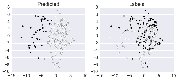
The GMM is poor at clustering rocks and mines based on the first 2 PC of the sonographic data.
np.corrcoef(predict, labels)
array([[ 1.        , -0.13825324],
       [-0.13825324,  1.        ]])
Plot discrepancy between predicted and labels
xs = np.array(features.collect()).squeeze()

fig, axes = plt.subplots(1, 2, figsize=(10, 4))
axes[0].scatter(xs[:, 0], xs[:,1], c=predict)
axes[0].set_title('Predicted')
axes[1].scatter(xs[:, 0], xs[:,1], c=labels)
axes[1].set_title('Labels')
pass
Supervised Learning
We will fit a logistic regression model to the data as an example of supervised learning.
sonar.show(n=3)
+--------------------+-----+---------+
|        std_features|label|label_idx|
+--------------------+-----+---------+
|[-0.3985897356694...|    R|      1.0|
|[0.70184498705605...|    R|      1.0|
|[-0.1289179854363...|    R|      1.0|
+--------------------+-----+---------+
only showing top 3 rows
Using mllib and RDDs
Convert to format expected by regression functions in mllib
data = sonar.map(lambda x: LabeledPoint(x[2], x[0]))
Split into test and train sets
train, test = data.randomSplit([0.7, 0.3])
Fit model to training data
model = LogisticRegressionWithLBFGS.train(train)
Evaluate on test data
y_yhat = test.map(lambda x: (x.label, model.predict(x.features)))
err = y_yhat.filter(lambda x: x[0] != x[1]).count() / float(test.count())
print("Error = " + str(err))
Error = 0.26229508196721313
Using the newer ml pipeline
transformer = VectorAssembler(inputCols=['C%d' % i for i in range(60)],
                              outputCol="features")
standardizer = StandardScaler(withMean=True, withStd=True,
                              inputCol='features',
                              outputCol='std_features')
indexer = StringIndexer(inputCol="C60", outputCol="label_idx")
pca = PCA(k=5, inputCol="std_features", outputCol="pca")
lr = LogisticRegression(featuresCol='std_features', labelCol='label_idx')

pipeline = Pipeline(stages=[transformer, standardizer, indexer, pca, lr])
df = (sqlc.read.format('com.databricks.spark.csv')
      .options(header='false', inferschema='true')
      .load('data/sonar.all-data.txt'))
train, test = df.randomSplit([0.7, 0.3])
model = pipeline.fit(train)
import warnings

with warnings.catch_warnings():
    warnings.simplefilter('ignore')
    prediction = model.transform(test)
score = prediction.select(['label_idx', 'prediction'])
score.show(n=score.count())
+---------+----------+
|label_idx|prediction|
+---------+----------+
|      0.0|       0.0|
|      0.0|       0.0|
|      0.0|       0.0|
|      0.0|       0.0|
|      0.0|       0.0|
|      0.0|       0.0|
|      0.0|       0.0|
|      0.0|       0.0|
|      0.0|       1.0|
|      0.0|       0.0|
|      0.0|       0.0|
|      0.0|       1.0|
|      0.0|       0.0|
|      0.0|       1.0|
|      0.0|       0.0|
|      0.0|       0.0|
|      0.0|       0.0|
|      0.0|       1.0|
|      0.0|       0.0|
|      1.0|       0.0|
|      0.0|       0.0|
|      0.0|       0.0|
|      0.0|       1.0|
|      1.0|       0.0|
|      1.0|       1.0|
|      1.0|       0.0|
|      0.0|       0.0|
|      1.0|       1.0|
|      1.0|       1.0|
|      1.0|       1.0|
|      1.0|       1.0|
|      1.0|       1.0|
|      1.0|       1.0|
|      1.0|       1.0|
|      1.0|       0.0|
|      1.0|       1.0|
|      1.0|       0.0|
|      1.0|       1.0|
|      1.0|       1.0|
|      1.0|       1.0|
|      1.0|       1.0|
|      1.0|       1.0|
|      1.0|       1.0|
|      1.0|       1.0|
|      1.0|       1.0|
|      1.0|       1.0|
|      1.0|       1.0|
|      1.0|       1.0|
|      1.0|       0.0|
|      1.0|       0.0|
|      1.0|       1.0|
|      1.0|       1.0|
|      1.0|       0.0|
|      1.0|       1.0|
|      1.0|       1.0|
|      1.0|       1.0|
|      1.0|       0.0|
|      1.0|       0.0|
|      1.0|       1.0|
|      1.0|       1.0|
|      1.0|       1.0|
|      1.0|       1.0|
|      1.0|       1.0|
|      1.0|       1.0|
+---------+----------+
acc = score.map(lambda x: x[0] == x[1]).sum() / score.count()
acc
0.765625
Spark MLLIb and sklearn integration
There is a package that you can install with
pip install spark-sklearn
Basically, it provides the same API as sklearn but uses Spark MLLib
under the hood to perform the actual computations in a distributed way
(passed in via the SparkContext instance).
Example taken directly from package website
Install if necessary
! pip install spark_sklearn
from sklearn import svm, grid_search, datasets
from spark_sklearn import GridSearchCV
iris = datasets.load_iris()
parameters = {'kernel':('linear', 'rbf'), 'C':[1, 10]}
svr = svm.SVC()
clf = GridSearchCV(sc, svr, parameters)
clf.fit(iris.data, iris.target)
GridSearchCV(cv=None, error_score='raise',
       estimator=SVC(C=1.0, cache_size=200, class_weight=None, coef0=0.0,
  decision_function_shape=None, degree=3, gamma='auto', kernel='rbf',
  max_iter=-1, probability=False, random_state=None, shrinking=True,
  tol=0.001, verbose=False),
       fit_params={}, iid=True, n_jobs=1,
       param_grid={'kernel': ('linear', 'rbf'), 'C': [1, 10]},
       pre_dispatch='2*n_jobs', refit=True,
       sc=<pyspark.context.SparkContext object at 0x10435ef60>,
       scoring=None, verbose=0)