6. 8 Durham: Income, Trees, & Temps
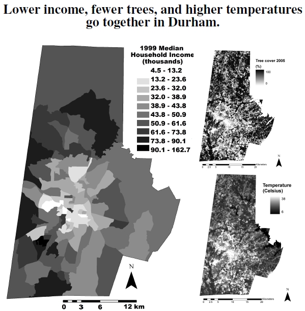
 Figure 6.8: At left, Durham County’s median income levels averaged over Year 2000 U.S. Census block groups (by Rob Schick). On the right, for easy comparison, are the canopy fraction (top right) and temperature profile (bottom right), previously shown and discussed in Figure 2.1. Visually, a positive correlation appears between median income and canopy cover, and a negative correlation between median income and temperature. Figure 6.13 quantifies this correlation.
The remainder of this chapter examines the benefits and distribution of urban vegetation. The images in Figure 6.8 display Year 2000 median income levels in Durham, North Carolina, averaged across census blocks, the large image at left, along with the previously discussed tree cover (top right) and temperature profiles (bottom right) across the county (see Figure 2.1). Light areas indicate low income, low tree cover, and high temperature, respectively. Visual inspection, at least by my eye, shows that all three images reflect one another, meaning that the different variables correlate with one another. For example, the lightly shaded lower-income area, just to the lower left of the city center, shows up clearly in the other two images as a high temperature and low canopy cover region. Similarly, a dark area in the northern part of the county, indicating high income, corresponds to a particularly high-income development near a watershed area having high canopy cover and low temperature. Indeed, statistical analysis presented later in this chapter (see Figure 6.13) bears out these apparent correlations: With wealth comes extensive tree canopy cover and lower temperatures.
I’m not picking on Durham: I love Durham. As I show throughout this chapter, however, environmental inequities exist throughout the United States and the world. Income–vegetation–temperature correlations materialize in many different ways across many urban areas. For example, canopy cover maps in Denver, Colorado, showed that both commercial land use and high population density correlate with low levels of vegetation.[31] Those correlations make simple common sense. To make a new building, you first have to remove grass and trees. Beyond these factors, other land-use types had complicated connections to vegetation. For example, neighborhood age generally implies higher vegetation, but features associated with small lots negate this tendency. Economically disadvantaged neighborhoods found near commercial areas had low vegetation. Sparsely populated areas with large lots owned by wealthy white people had particularly high correlations with vegetation.
I live in an area just north of the city of Durham, where, seemingly, zoning laws forbid commercial and retail activities, perhaps as a way to inhibit sprawl, or perhaps because people prefer to live far from retail spaces if they can afford it (see Figure 5.3).[32] As a result, these areas have fewer impervious parking lots, larger residential lots, lower temperatures, and fewer economic or open space disadvantages. Of course, the trade-off means that residents must drive to the nearest store to buy that emergency gallon of milk. The real need for urban open space falls right where the economically disadvantaged folks live, where, surprise, there’s typically little open space.
—————————————–
31Mennis (2006) examined vegetation and socioeconomic variables in Denver, Colorado, using two different approaches: a standard multivariate regression and a novel rule-mining approach.
32Thompson (2002) states that changing the “pattern” of a city from a centralized one to compact neighborhoods or urban areas with hubs helps equity, and outlines several reasons to have this space available.