Computer numbers and mathematics¶

Some examples of numbers behaving badly¶

def normalize(ws):
    """Returns normalized set of weights that sum to 1."""
    s = sum(ws)
    return [w/s for w in ws]

ws = [1,2,3,4,5]
normalize(ws)

[0, 0, 0, 0, 0]

from scipy.stats import norm

rv1 = norm(0, 1)
rv2 = norm(0, 3)

xs = np.random.normal(0, 3, 1000)
likelihood1 = np.prod(rv1.pdf(xs))
likelihood2 = np.prod(rv2.pdf(xs))
likelihood2 > likelihood1

False

s = 0.0

for i in range(1000):
    s += 1.0/10.0
    if s == 1.0:
        break
print i

999

def var(xs):
    """Returns variance of sample data."""
    n = 0
    s = 0
    ss = 0

    for x in xs:
        n +=1
        s += x
        ss += x*x

    v = (ss - (s*s)/n)/(n-1)
    return v

# What is the sample variance for numbers from a normal distribution with variance 1?
np.random.seed(4)
xs = np.random.normal(1e9, 1, 1000)
var(xs)

-262.4064

Finite representation of numbers¶

For integers, there is a maximum and minimum representatble number for langauges. Python integers are acutally objects, so they intelligently switch to arbitrary precision numbers when you go beyond these limits, but this is not true for most other languages including C and R. With 64 bit representation, the maximumm is 2^63 - 1 and the minimum is -2^63 - 1.

import sys
sys.maxint

9223372036854775807

2**63-1 == sys.maxint

True

# Python handles "overflow" of integers gracefully by
# swithing from integers to "long" abritrary precsion numbers
sys.maxint + 1

9223372036854775808L

# Explicit float conversion

print float(1)/3

0.333333333333

# Implicit float conversion

print (0.0 + 1)/3
print (1.0 * 1)/3

0.333333333333
0.333333333333

# Telling Python to ALWAYS do floaitng point with '/'
# Integer division can still be done with '//'
# The __futre__ package contains routines that are only
# found beyond some Python release number.

from __future__ import division

print (1/3)
print (1//3)

0.333333333333
0

sudo apt-get update
sudo apt-get install build-essential
sudo apt-get install llvm
pip install git+https://github.com/dabeaz/bitey.git

%%file demo.c

#include "limits.h"

long limit() {
    return LONG_MAX;
}

long overflow() {
    long x = LONG_MAX;
    return x+1;
}

Writing demo.c

! clang -emit-llvm -c demo.c -o demo.o

import bitey
import demo

demo.limit(), demo.overflow()

(9223372036854775807, -9223372036854775808)

Floating point numbers¶

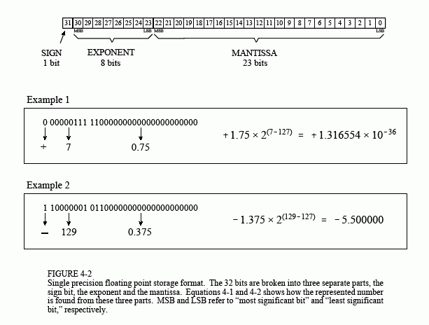
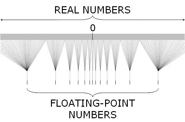
A floating point number is stored in 3 pieces (sign bit, exponent, mantissa) so that every float is represetned as get +/- mantissa ^ exponent. Because of this, the interval between consecutive numbers is smallest (high precison) for numebrs close to 0 and largest for numbers close to the lower and upper bounds.

Because exponents have to be singed to represent both small and large numbers, but it is more convenint to use unsigned numbers here, the exponnent has an offset (also knwnn as the exponentn bias). For example, if the expoennt is an unsigned 8-bit number, it can rerpesent the range (0, 255). By using an offset of 128, it will now represent the range (-127, 128).

from IPython.display import Image

Binary represetnation of a floating point number¶

Image(url='http://www.dspguide.com/graphics/F_4_2.gif')

Intervals between consecutive floating point numbers are not constant¶

Because of this, if you are adding many numbers, it is more accuate to first add the small numbers before the large numbers.

Image(url='http:///fig1.jpg')

Floating point numbers on your system¶

Information about the floating point reresentation on your system can be obtained from sys.float_info. Definitions of the stored values are given at https://docs.python.org/2/library/sys.html#sys.float_info

import sys

print sys.float_info

sys.float_info(max=1.7976931348623157e+308, max_exp=1024, max_10_exp=308, min=2.2250738585072014e-308, min_exp=-1021, min_10_exp=-307, dig=15, mant_dig=53, epsilon=2.220446049250313e-16, radix=2, rounds=1)

Floating point numbers may not be precise¶

'%.20f' % (0.1 * 0.1 * 100)

'1.00000000000000022204'

# Because of this, don't chek for equality of floating point numbers!

# Bad
s = 0.0

for i in range(1000):
    s += 1.0/10.0
    if s == 1.0:
        break
print i

# OK

TOL = 1e-9
s = 0.0

for i in range(1000):
    s += 1.0/10.0
    if abs(s - 1.0) < TOL:
        break
print i

999
9

# Loss of precision
1 + 6.022e23 - 6.022e23

0.0000

Lesson: Avoid algorithms that subtract two numbers that are very close to one anotoer. The loss of significnance is greater when both numbers are very large due to the limited number of precsion bits available.

Associative law does not necessarily hold¶

6.022e23 - 6.022e23 + 1

1.0000

1 + 6.022e23 - 6.022e23

0.0000

Distributive law does not hold¶

a = np.exp(1);
b = np.pi;
c = np.sin(1);
a*(b+c) == a*b+a*c

False

# loss of precision can be a problem when calculating likelihoods
probs = np.random.random(1000)
np.prod(probs)

0.0000

# when multiplying lots of small numbers, work in log space
np.sum(np.log(probs))

-980.0558

Lesson: Work in log space for very small or very big numbers to reduce underflow/overflow

Using arbitrary precision libraries¶

If you need precision more than speed (e.g. your code is likely to underflow or overflow otherwise and you cannot find or don’t want to use a workaround), Python has support for arbitrary precison mathematics via

• The decimal package in th standard library
• The mpmath package
• The gmpy2 package

Both mpmath and gmpy2 can be installed via pip

pip install gmpy2
pip install mpmath

These packages allow you to set the precsion of numbers used in calculations. Refer to the documentation if you need to use these libraries.

From numbers to Functions: Stability and conditioning¶

Suppose we have a computer algorithm \(g(x)\) that represents the mathematical function \(f(x)\). \(g(x)\) is stable if for some small perturbation \(\epsilon\), \(g(x+\epsilon) \approx f(x)\)

A mathematical function \(f(x)\) is well-conditioned if \(f(x + \epsilon) \approx f(x)\) for all small perturbations \(\epsilon\).

That is, the function\(f(x)\) is well-conditioned if the solution varies gradually as problem varies. For a well-conditinoed function, all small perutbations have small effects. However, a poorly-conditioned problem only needs some small perturbations to have large effects. For example, inverting a nearly singluar matrix is a poorly condiitioned problem.

A numerical algorithm \(g(x)\) is numerically-stable if \(g(x) \approx f(x')\) for some \(x' \approx x\). Note that stability is a property that relates the algorithm \(g(x)\) to the problem \(f(x)\).

That is, the algorithm\(g(x)\) is numerically stable if it gives nearly the right answer to nearly the right question. Numerically unstable algorithms tend to amplify approximation errors due to computer arithmetic over time. If we used an infitinte precision numerical system, stable and unstable alorithms would have the same accuracy. However, as we have seen (e.g. variance calculation), when using floating point numbers, algebrically equivaelent algorithms can give different results.

In general, we need both a well-conditinoed problem and nuerical stabilty of the algorihtm to reliably accurate answers. In this case, we can be sure that \(g(x) \approx f(x)\).

Unstable version

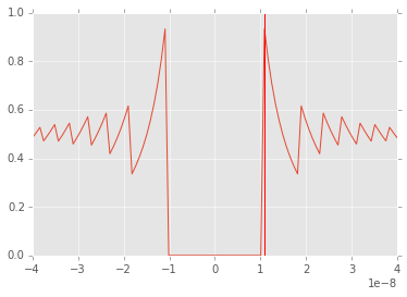
# Catastrophic cancellation occurs when subtracitng
# two numbers that are very close to one another
# Here is another example

def f(x):
    return (1 - np.cos(x))/(x*x)

x = np.linspace(-4e-8, 4e-8, 100)
plt.plot(x,f(x));
plt.axvline(1.1e-8, color='red')
plt.xlim([-4e-8, 4e-8]);

# We know from L'Hopital's rule that the answer is 0.5 at 0
# and should be very close to 0.5 throughout this tiny interval
# but errors arisee due to catastrophic cancellation

print '%.30f' % np.cos(1.1e-8)
print '%.30f' % (1 - np.cos(1.1e-8)) # exact answer is 6.05e-17
print '%2f' % ((1 - np.cos(1.1e-8))/(1.1e-8*1.1e-8))

0.999999999999999888977697537484
0.000000000000000111022302462516
0.917540

Stable version

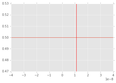
# Numerically stable version of funtion
# using long-forgotten half-angle formula from trignometry

def f1(x):
    return 2*np.sin(x/2)**2/(x*x)

x = np.linspace(-4e-8, 4e-8, 100)
plt.plot(x,f1(x));
plt.axvline(1.1e-8, color='red')
plt.xlim([-4e-8, 4e-8]);

# sum of squares method (vectorized version)
def sum_of_squers_var(x):
    n = len(x)
    return (1.0/(n*(n-1))*(n*np.sum(x**2) - (np.sum(x))**2))

# direct method
def direct_var(x):
    n = len(x)
    xbar = np.mean(x)
    return 1.0/(n-1)*np.sum((x - xbar)**2)

# Welford's method
def welford_var(x):
    s = 0
    m = x[0]
    for i in range(1, len(x)):
        m += (x[i]-m)/i
        s += (x[i]-m)**2
    return s/(len(x) -1 )

x_ = np.random.uniform(0,1,1e6)
x = 1e12 + x_

# correct answer
np.var(x_)

0.0835

sum_of_squers_var(x)

737870500.8189

direct_var(x)

0.0835

welford_var(x)

0.0835

np.log(x + 1)

np.log1p(x)

np.sin(x)/x

np.sinc(x)

# The tangent function is poorly conditioned

x1 = 1.57078
x2 = 1.57079
t1 = np.tan(x1)
t2 = np.tan(x2)

print 't1 =', t1
print 't2 =', t2
print '% change in x =', 100.0*(x2-x1)/x1
print '% change in tan(x) =', (100.0*(t2-t1)/t1)

t1 = 61249.0085315
t2 = 158057.913416
% change in x = 0.000636626389427
% change in tan(x) = 158.057913435

A = 0.5*np.array([[1,1], [1+1e-10, 1-1e-10]])
b1 = np.array([2,2])
b2 = np.array([2.01, 2])

np.linalg.solve(A, b1)

array([ 2.,  2.])

np.linalg.solve(A, b2)

array([-99999989.706,  99999993.726])

np.linalg.cond(A)

19999973849.2252

np.linalg.cond(A, 'fro')

19999998343.1927

Exercises¶

The topic is rather specialized and the main goal is just to have you aware of the “leaky abstraction” of computer numbers as simulations of mathematical numbers, and common situations where this can casue problems. Once you are aware of these areas, you can either avoid them using simple rules, or look for an apprpriate numerical library fuctionn to use instead. So there will be no exericses on the topic of computer arithmetic, conditioning and stability given.

Instead, you need to get as comforatble with the use of arrays in numpy as much as possible for the rest of the course. For practice, see the entertaining examples and exercises at

Nicolas P. Rougier’s numpy tutorial

At the end, there are further links to yet more numpy tutorials!