import os
import sys
import glob
import matplotlib.pyplot as plt
import numpy as np
import pandas as pd
%matplotlib inline
plt.style.use('ggplot')
np.random.seed(1234)

np.set_printoptions(formatter={'all':lambda x: '%.3f' % x})
from IPython.display import Image
from numpy.core.umath_tests import matrix_multiply as mm
from scipy.optimize import minimize
from scipy.stats import bernoulli, binom
Expectation Maximizatio (EM) Algorithm
- Review of Jensen’s inequality
- Concavity of log function
- Example of coin tossing with missing informaiton to provide context
- Derivation of EM equations
- Illustration of EM convergence
- Derivation of update equations of coin tossing example
- Code for coin tossing example
- Derivation of update equatiosn for mixture of Gaussians
- Code for mixture of Gaussians
Jensen’s inequality
For a convex function \(f\), \(E[f(x)] \geq f(E[x])\). Flip the sign for a concave function.
A function \(f(x)\) is convex if \(f''(x) \geq 0\) everywhere in its domain. For example, if \(f(x) = \log x\), \(f''(x) = -1/x^2\), so the log function is concave for \(x \in (0, \infty]\). A visual illustration of Jensen’s inequality is shown below.
Image(filename='figs/jensen.png')
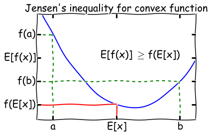
When is Jensen’s inequality an equality? From the diagram, we can see that this only happens if the function \(f(x)\) is a constant! We will make use of this fact later on in the lecture.
Maximum likelihood with complete information
Consider an experiment with coin \(A\) that has a probability \(\theta_A\) of heads, and a coin \(B\) that has a probability \(\theta_B\) of tails. We draw \(m\) samples as follows - for each sample, pick one of the coins at random, flip it \(n\) times, and record the number of heads and tails (that sum to \(n\)). If we recorded which coin we used for each sample, we have complete information and can estimate \(\theta_A\) and \(\theta_B\) in closed form. To be very explicit, suppose we drew 5 samples with the number of heads and tails represented as a vector \(x\), and the sequence of coins chosen was \(A, A, B, A, B\). Then the complete log likelihood is
where \(p(x_i; \theta)\) is the binomial distribtion PMF with \(n=m\) and \(p=\theta\). We will use \(z_i\) to indicate the label of the \(i^\text{th}\) coin, that is - whether we used coin \(A\) or \(B\) to gnerate the \(i^\text{th}\) sample.
Coin toss example from What is the expectation maximization algorithm?
Solving for complete likelihood using minimization
def neg_loglik(thetas, n, xs, zs):
    return -np.sum([binom(n, thetas[z]).logpmf(x) for (x, z) in zip(xs, zs)])
m = 10
theta_A = 0.8
theta_B = 0.3
theta_0 = [theta_A, theta_B]

coin_A = bernoulli(theta_A)
coin_B = bernoulli(theta_B)

xs = map(sum, [coin_A.rvs(m), coin_A.rvs(m), coin_B.rvs(m), coin_A.rvs(m), coin_B.rvs(m)])
zs = [0, 0, 1, 0, 1]
Exact solution
xs = np.array(xs)
xs
array([7.000, 9.000, 2.000, 6.000, 0.000])
ml_A = np.sum(xs[[0,1,3]])/(3.0*m)
ml_B = np.sum(xs[[2,4]])/(2.0*m)
ml_A, ml_B
(0.73333333333333328, 0.10000000000000001)
Numerical estimate
bnds = [(0,1), (0,1)]
minimize(neg_loglik, [0.5, 0.5], args=(m, xs, zs),
         bounds=bnds, method='tnc', options={'maxiter': 100})
 status: 1
success: True
   nfev: 17
    fun: 7.6552677541393193
      x: array([0.733, 0.100])
message: 'Converged (|f_n-f_(n-1)| ~= 0)'
    jac: array([-0.000, -0.000])
    nit: 6
Incomplete information
However, if we did not record the coin we used, we have missing data and the problem of estimating \(\theta\) is harder to solve. One way to approach the problem is to ask - can we assign weights \(w_i\) to each sample according to how likely it is to be generated from coin \(A\) or coin \(B\)?
With knowledge of \(w_i\), we can maximize the likelihod to find \(\theta\). Similarly, given \(w_i\), we can calculate what \(\theta\) should be. So the basic idea behind Expectation Maximization (EM) is simply to start with a guess for \(\theta\), then calculate \(z\), then update \(\theta\) using this new value for \(z\), and repeat till convergence. The derivation below shows why the EM algorithm using this “alternating” updates actually works.
A verbal outline of the derivtion - first consider the log likelihood function as a curve (surface) where the base is \(\theta\). Find another function \(Q\) of \(\theta\) that is a lower bound of the log-likelihood but touches the log likelihodd function at some \(\theta\) (E-step). Next find the value of \(\theta\) that maximizes this function (M-step). Now find yet antoher function of \(\theta\) that is a lower bound of the log-likelihood but touches the log likelihodd function at this new \(\theta\). Now repeat until convergence - at this point, the maxima of the lower bound and likelihood functions are the same and we have found the maximum log likelihood. See illustratioin below.
# Image from http://www.nature.com/nbt/journal/v26/n8/extref/nbt1406-S1.pdf
Image(filename='figs/em.png', width=800)

The only remaining step is how to find the functions that are lower bounds of the log likelihood. This will require a little math using Jensen’s inequality, and is shown in the next section.
In the E-step, we identify a function which is a lower bound for the log-likelikelihood
How do we choose the distribution \(Q_i\)? We want the Q function to touch the log-likelihood, and know that Jensen’s inequality is an equality only if the function is constant. So
So \(Q_i\) is just the posterior distribution of \(z_i\), and this completes the E-step.
In the M-step, we find the value of \(\theta\) that maximizes the Q function, and then we iterate over the E and M steps until convergence.
So we see that EM is an algorihtm for maximum likelikhood optimization when there is missing inforrmaiton - or when it is useful to add latent augmented variables to simplify maximum likelihood calculatoins.
- \(i\) indicates the sample
- \(j\) indicates the coin
- \(l\) is an index running through each of the coins
- \(\theta\) is the probability of the coin being heads
- \(\phi\) is the probability of choosing a particular coin
- \(h\) is the number of heads in a sample
- \(n\) is the number of coin tosses in a sample
- \(k\) is the number of coins
- \(m\) is the number of samples
For the E-step, with each sample we have
For the M-step, we need to find the value of \(\theta\) that maximises the \(Q\) function
We can differentiate and solve for each component \(\theta_s\) where the derivative vanishes
xs = np.array([(5,5), (9,1), (8,2), (4,6), (7,3)])
thetas = np.array([[0.6, 0.4], [0.5, 0.5]])

tol = 0.01
max_iter = 100

ll_old = 0
for i in range(max_iter):
    ws_A = []
    ws_B = []

    vs_A = []
    vs_B = []

    ll_new = 0

    # E-step: calculate probability distributions over possible completions
    for x in xs:

        # multinomial (binomial) log likelihood
        ll_A = np.sum([x*np.log(thetas[0])])
        ll_B = np.sum([x*np.log(thetas[1])])

        # [EQN 1]
        denom = np.exp(ll_A) + np.exp(ll_B)
        w_A = np.exp(ll_A)/denom
        w_B = np.exp(ll_B)/denom

        ws_A.append(w_A)
        ws_B.append(w_B)

        # used for calculating theta
        vs_A.append(np.dot(w_A, x))
        vs_B.append(np.dot(w_B, x))

        # update complete log likelihood
        ll_new += w_A * ll_A + w_B * ll_B

    # M-step: update values for parameters given current distribution
    # [EQN 2]
    thetas[0] = np.sum(vs_A, 0)/np.sum(vs_A)
    thetas[1] = np.sum(vs_B, 0)/np.sum(vs_B)
    # print distribution of z for each x and current parameter estimate

    print "Iteration: %d" % (i+1)
    print "theta_A = %.2f, theta_B = %.2f, ll = %.2f" % (thetas[0,0], thetas[1,0], ll_new)

    if np.abs(ll_new - ll_old) < tol:
        break
    ll_old = ll_new
Iteration: 1
theta_A = 0.71, theta_B = 0.58, ll = -32.69
Iteration: 2
theta_A = 0.75, theta_B = 0.57, ll = -31.26
Iteration: 3
theta_A = 0.77, theta_B = 0.55, ll = -30.76
Iteration: 4
theta_A = 0.78, theta_B = 0.53, ll = -30.33
Iteration: 5
theta_A = 0.79, theta_B = 0.53, ll = -30.07
Iteration: 6
theta_A = 0.79, theta_B = 0.52, ll = -29.95
Iteration: 7
theta_A = 0.80, theta_B = 0.52, ll = -29.90
Iteration: 8
theta_A = 0.80, theta_B = 0.52, ll = -29.88
Iteration: 9
theta_A = 0.80, theta_B = 0.52, ll = -29.87
xs = np.array([(5,5), (9,1), (8,2), (4,6), (7,3)])
thetas = np.array([[0.6, 0.4], [0.5, 0.5]])

tol = 0.01
max_iter = 100

ll_old = -np.infty
for i in range(max_iter):
    ll_A = np.sum(xs * np.log(thetas[0]), axis=1)
    ll_B = np.sum(xs * np.log(thetas[1]), axis=1)
    denom = np.exp(ll_A) + np.exp(ll_B)
    w_A = np.exp(ll_A)/denom
    w_B = np.exp(ll_B)/denom

    vs_A = w_A[:, None] * xs
    vs_B = w_B[:, None] * xs

    thetas[0] = np.sum(vs_A, 0)/np.sum(vs_A)
    thetas[1] = np.sum(vs_B, 0)/np.sum(vs_B)

    ll_new = w_A.dot(ll_A) + w_B.dot(ll_B)

    print "Iteration: %d" % (i+1)
    print "theta_A = %.2f, theta_B = %.2f, ll = %.2f" % (thetas[0,0], thetas[1,0], ll_new)

    if np.abs(ll_new - ll_old) < tol:
        break
    ll_old = ll_new
Iteration: 1
theta_A = 0.71, theta_B = 0.58, ll = -32.69
Iteration: 2
theta_A = 0.75, theta_B = 0.57, ll = -31.26
Iteration: 3
theta_A = 0.77, theta_B = 0.55, ll = -30.76
Iteration: 4
theta_A = 0.78, theta_B = 0.53, ll = -30.33
Iteration: 5
theta_A = 0.79, theta_B = 0.53, ll = -30.07
Iteration: 6
theta_A = 0.79, theta_B = 0.52, ll = -29.95
Iteration: 7
theta_A = 0.80, theta_B = 0.52, ll = -29.90
Iteration: 8
theta_A = 0.80, theta_B = 0.52, ll = -29.88
Iteration: 9
theta_A = 0.80, theta_B = 0.52, ll = -29.87
xs = np.array([(5,5), (9,1), (8,2), (4,6), (7,3)])
thetas = np.array([[0.6, 0.4], [0.5, 0.5]])

tol = 0.01
max_iter = 100

ll_old = -np.infty
for i in range(max_iter):
    ll_A = np.sum(xs * np.log(thetas[0]), axis=1)
    ll_B = np.sum(xs * np.log(thetas[1]), axis=1)
    denom = np.exp(ll_A) + np.exp(ll_B)
    w_A = np.exp(ll_A)/denom
    w_B = np.exp(ll_B)/denom

    vs_A = w_A[:, None] * xs
    vs_B = w_B[:, None] * xs

    thetas[0] = np.sum(vs_A, 0)/np.sum(vs_A)
    thetas[1] = np.sum(vs_B, 0)/np.sum(vs_B)

    ll_new = w_A.dot(ll_A) + w_B.dot(ll_B) - w_A.dot(np.log(w_A)) - w_B.dot(np.log(w_B))

    print "Iteration: %d" % (i+1)
    print "theta_A = %.2f, theta_B = %.2f, ll = %.2f" % (thetas[0,0], thetas[1,0], ll_new)

    if np.abs(ll_new - ll_old) < tol:
        break
    ll_old = ll_new
Iteration: 1
theta_A = 0.71, theta_B = 0.58, ll = -29.63
Iteration: 2
theta_A = 0.75, theta_B = 0.57, ll = -28.39
Iteration: 3
theta_A = 0.77, theta_B = 0.55, ll = -28.26
Iteration: 4
theta_A = 0.78, theta_B = 0.53, ll = -28.16
Iteration: 5
theta_A = 0.79, theta_B = 0.53, ll = -28.12
Iteration: 6
theta_A = 0.79, theta_B = 0.52, ll = -28.11
Iteration: 7
theta_A = 0.80, theta_B = 0.52, ll = -28.10
def em(xs, thetas, max_iter=100, tol=1e-6):
    """Expectation-maximization for coin sample problem."""

    ll_old = -np.infty
    for i in range(max_iter):
        ll = np.array([np.sum(xs * np.log(theta), axis=1) for theta in thetas])
        lik = np.exp(ll)
        ws = lik/lik.sum(0)
        vs = np.array([w[:, None] * xs for w in ws])
        thetas = np.array([v.sum(0)/v.sum() for v in vs])
        ll_new = np.sum([w*l for w, l in zip(ws, ll)])
        if np.abs(ll_new - ll_old) < tol:
            break
        ll_old = ll_new
    return i, thetas, ll_new
xs = np.array([(5,5), (9,1), (8,2), (4,6), (7,3)])
thetas = np.array([[0.6, 0.4], [0.5, 0.5]])

i, thetas, ll = em(xs, thetas)
print i
for theta in thetas:
    print theta
print ll
np.random.seed(1234)

n = 100
p0 = 0.8
p1 = 0.35
xs = np.concatenate([np.random.binomial(n, p0, n/2), np.random.binomial(n, p1, n/2)])
xs = np.column_stack([xs, n-xs])
np.random.shuffle(xs)
results = [em(xs, np.random.random((2,2))) for i in range(10)]
i, thetas, ll =  sorted(results, key=lambda x: x[-1])[-1]
print i
for theta in thetas:
    print theta
print ll
Gaussian mixture models
import scipy.stats as st
def f(x, y):
    z = np.column_stack([x.ravel(), y.ravel()])
    return (0.1*st.multivariate_normal([0,0], 1*np.eye(2)).pdf(z) +
            0.4*st.multivariate_normal([3,3], 2*np.eye(2)).pdf(z) +
            0.5*st.multivariate_normal([0,5], 3*np.eye(2)).pdf(z))
f(np.arange(3), np.arange(3))
s = 200
x = np.linspace(-3, 6, s)
y = np.linspace(-3, 8, s)
X, Y = np.meshgrid(x, y)
Z = np.reshape(f(X, Y), (s, s))

from mpl_toolkits.mplot3d import Axes3D
fig = plt.figure(figsize=(12,8))
ax = fig.add_subplot(111, projection='3d')
ax.plot_surface(X, Y, Z, cmap='jet')
plt.title('Gaussian Mxixture Model');
A mixture of \(k\) Gaussians has the following PDF
where \(\alpha_j\) is the weight of the \(j^\text{th}\) Gaussain component and
Suppose we observe \(y_1, y_2, \ldots, y_n\) as a sample from a mixture of Gaussians. The log-likeihood is then
where \(\theta = (\alpha, \mu, \Sigma)\)
There is no closed form for maximizing the parameters of this log-likelihood, and it is hard to maximize directly.
Using EM
Suppose we augment with the latent variable \(z\) that indicates which of the \(k\) Gaussians our observation \(y\) came from. The derivation of the E and M steps are the same as for the toy example, only with more algebra.
For the E-step, we have
For the M-step, we have to find \(\theta = (w, \mu, \Sigma)\) that maximizes \(Q\)
By taking derivatives with respect to \((w, \mu, \Sigma)\) respectively and solving (remember to use Lagrange multipliers for the constraint that \(\sum_{j=1}^k w_j = 1\)), we get
from scipy.stats import multivariate_normal as mvn
def em_gmm_orig(xs, pis, mus, sigmas, tol=0.01, max_iter=100):

    n, p = xs.shape
    k = len(pis)

    ll_old = 0
    for i in range(max_iter):
        exp_A = []
        exp_B = []
        ll_new = 0

        # E-step
        ws = np.zeros((k, n))
        for j in range(len(mus)):
            for i in range(n):
                ws[j, i] = pis[j] * mvn(mus[j], sigmas[j]).pdf(xs[i])
        ws /= ws.sum(0)

        # M-step
        pis = np.zeros(k)
        for j in range(len(mus)):
            for i in range(n):
                pis[j] += ws[j, i]
        pis /= n

        mus = np.zeros((k, p))
        for j in range(k):
            for i in range(n):
                mus[j] += ws[j, i] * xs[i]
            mus[j] /= ws[j, :].sum()

        sigmas = np.zeros((k, p, p))
        for j in range(k):
            for i in range(n):
                ys = np.reshape(xs[i]- mus[j], (2,1))
                sigmas[j] += ws[j, i] * np.dot(ys, ys.T)
            sigmas[j] /= ws[j,:].sum()

        # update complete log likelihoood
        ll_new = 0.0
        for i in range(n):
            s = 0
            for j in range(k):
                s += pis[j] * mvn(mus[j], sigmas[j]).pdf(xs[i])
            ll_new += np.log(s)

        if np.abs(ll_new - ll_old) < tol:
            break
        ll_old = ll_new

    return ll_new, pis, mus, sigmas
Vectorized version
def em_gmm_vect(xs, pis, mus, sigmas, tol=0.01, max_iter=100):

    n, p = xs.shape
    k = len(pis)

    ll_old = 0
    for i in range(max_iter):
        exp_A = []
        exp_B = []
        ll_new = 0

        # E-step
        ws = np.zeros((k, n))
        for j in range(k):
            ws[j, :] = pis[j] * mvn(mus[j], sigmas[j]).pdf(xs)
        ws /= ws.sum(0)

        # M-step
        pis = ws.sum(axis=1)
        pis /= n

        mus = np.dot(ws, xs)
        mus /= ws.sum(1)[:, None]

        sigmas = np.zeros((k, p, p))
        for j in range(k):
            ys = xs - mus[j, :]
            sigmas[j] = (ws[j,:,None,None] * mm(ys[:,:,None], ys[:,None,:])).sum(axis=0)
        sigmas /= ws.sum(axis=1)[:,None,None]

        # update complete log likelihoood
        ll_new = 0
        for pi, mu, sigma in zip(pis, mus, sigmas):
            ll_new += pi*mvn(mu, sigma).pdf(xs)
        ll_new = np.log(ll_new).sum()

        if np.abs(ll_new - ll_old) < tol:
            break
        ll_old = ll_new

    return ll_new, pis, mus, sigmas
Vectorization with Einstein summation notation
def em_gmm_eins(xs, pis, mus, sigmas, tol=0.01, max_iter=100):

    n, p = xs.shape
    k = len(pis)

    ll_old = 0
    for i in range(max_iter):
        exp_A = []
        exp_B = []
        ll_new = 0

        # E-step
        ws = np.zeros((k, n))
        for j, (pi, mu, sigma) in enumerate(zip(pis, mus, sigmas)):
            ws[j, :] = pi * mvn(mu, sigma).pdf(xs)
        ws /= ws.sum(0)

        # M-step
        pis = np.einsum('kn->k', ws)/n
        mus = np.einsum('kn,np -> kp', ws, xs)/ws.sum(1)[:, None]
        sigmas = np.einsum('kn,knp,knq -> kpq', ws,
            xs-mus[:,None,:], xs-mus[:,None,:])/ws.sum(axis=1)[:,None,None]

        # update complete log likelihoood
        ll_new = 0
        for pi, mu, sigma in zip(pis, mus, sigmas):
            ll_new += pi*mvn(mu, sigma).pdf(xs)
        ll_new = np.log(ll_new).sum()

        if np.abs(ll_new - ll_old) < tol:
            break
        ll_old = ll_new

    return ll_new, pis, mus, sigmas
Comparison of EM routines
np.random.seed(123)

# create data set
n = 1000
_mus = np.array([[0,4], [-2,0]])
_sigmas = np.array([[[3, 0], [0, 0.5]], [[1,0],[0,2]]])
_pis = np.array([0.6, 0.4])
xs = np.concatenate([np.random.multivariate_normal(mu, sigma, int(pi*n))
                    for pi, mu, sigma in zip(_pis, _mus, _sigmas)])

# initial guesses for parameters
pis = np.random.random(2)
pis /= pis.sum()
mus = np.random.random((2,2))
sigmas = np.array([np.eye(2)] * 2)
%%time
ll1, pis1, mus1, sigmas1 = em_gmm_orig(xs, pis, mus, sigmas)
intervals = 101
ys = np.linspace(-8,8,intervals)
X, Y = np.meshgrid(ys, ys)
_ys = np.vstack([X.ravel(), Y.ravel()]).T

z = np.zeros(len(_ys))
for pi, mu, sigma in zip(pis1, mus1, sigmas1):
    z += pi*mvn(mu, sigma).pdf(_ys)
z = z.reshape((intervals, intervals))

ax = plt.subplot(111)
plt.scatter(xs[:,0], xs[:,1], alpha=0.2)
plt.contour(X, Y, z, N=10)
plt.axis([-8,6,-6,8])
ax.axes.set_aspect('equal')
plt.tight_layout()
%%time
ll2, pis2, mus2, sigmas2 = em_gmm_vect(xs, pis, mus, sigmas)
intervals = 101
ys = np.linspace(-8,8,intervals)
X, Y = np.meshgrid(ys, ys)
_ys = np.vstack([X.ravel(), Y.ravel()]).T

z = np.zeros(len(_ys))
for pi, mu, sigma in zip(pis2, mus2, sigmas2):
    z += pi*mvn(mu, sigma).pdf(_ys)
z = z.reshape((intervals, intervals))

ax = plt.subplot(111)
plt.scatter(xs[:,0], xs[:,1], alpha=0.2)
plt.contour(X, Y, z, N=10)
plt.axis([-8,6,-6,8])
ax.axes.set_aspect('equal')
plt.tight_layout()
%%time
ll3, pis3, mus3, sigmas3 = em_gmm_eins(xs, pis, mus, sigmas)
# %timeit em_gmm_orig(xs, pis, mus, sigmas)
%timeit em_gmm_vect(xs, pis, mus, sigmas)
%timeit em_gmm_eins(xs, pis, mus, sigmas)
intervals = 101
ys = np.linspace(-8,8,intervals)
X, Y = np.meshgrid(ys, ys)
_ys = np.vstack([X.ravel(), Y.ravel()]).T

z = np.zeros(len(_ys))
for pi, mu, sigma in zip(pis3, mus3, sigmas3):
    z += pi*mvn(mu, sigma).pdf(_ys)
z = z.reshape((intervals, intervals))

ax = plt.subplot(111)
plt.scatter(xs[:,0], xs[:,1], alpha=0.2)
plt.contour(X, Y, z, N=10)
plt.axis([-8,6,-6,8])
ax.axes.set_aspect('equal')
plt.tight_layout()