Set up environment¶

In [1]:

source("pilot_config.R")

Loading tidyverse: ggplot2
Loading tidyverse: tibble
Loading tidyverse: tidyr
Loading tidyverse: readr
Loading tidyverse: purrr
Loading tidyverse: dplyr
Conflicts with tidy packages ---------------------------------------------------
filter(): dplyr, stats
lag():    dplyr, stats

Attaching package: ‘foreach’

The following objects are masked from ‘package:purrr’:

    accumulate, when

Loading required package: S4Vectors
Loading required package: stats4
Loading required package: BiocGenerics
Loading required package: parallel

Attaching package: ‘BiocGenerics’

The following objects are masked from ‘package:parallel’:

    clusterApply, clusterApplyLB, clusterCall, clusterEvalQ,
    clusterExport, clusterMap, parApply, parCapply, parLapply,
    parLapplyLB, parRapply, parSapply, parSapplyLB

The following objects are masked from ‘package:dplyr’:

    combine, intersect, setdiff, union

The following objects are masked from ‘package:stats’:

    IQR, mad, sd, var, xtabs

The following objects are masked from ‘package:base’:

    anyDuplicated, append, as.data.frame, cbind, colMeans, colnames,
    colSums, do.call, duplicated, eval, evalq, Filter, Find, get, grep,
    grepl, intersect, is.unsorted, lapply, lengths, Map, mapply, match,
    mget, order, paste, pmax, pmax.int, pmin, pmin.int, Position, rank,
    rbind, Reduce, rowMeans, rownames, rowSums, sapply, setdiff, sort,
    table, tapply, union, unique, unsplit, which, which.max, which.min


Attaching package: ‘S4Vectors’

The following objects are masked from ‘package:dplyr’:

    first, rename

The following object is masked from ‘package:tidyr’:

    expand

The following object is masked from ‘package:base’:

    expand.grid

Loading required package: IRanges

Attaching package: ‘IRanges’

The following objects are masked from ‘package:dplyr’:

    collapse, desc, slice

The following object is masked from ‘package:purrr’:

    reduce

Loading required package: GenomicRanges
Loading required package: GenomeInfoDb
Loading required package: SummarizedExperiment
Loading required package: Biobase
Welcome to Bioconductor

    Vignettes contain introductory material; view with
    'browseVignettes()'. To cite Bioconductor, see
    'citation("Biobase")', and for packages 'citation("pkgname")'.

Loading required package: DelayedArray
Loading required package: matrixStats

Attaching package: ‘matrixStats’

The following objects are masked from ‘package:Biobase’:

    anyMissing, rowMedians

The following object is masked from ‘package:dplyr’:

    count


Attaching package: ‘DelayedArray’

The following objects are masked from ‘package:matrixStats’:

    colMaxs, colMins, colRanges, rowMaxs, rowMins, rowRanges

The following object is masked from ‘package:base’:

    apply


Attaching package: ‘limma’

The following object is masked from ‘package:DESeq2’:

    plotMA

The following object is masked from ‘package:BiocGenerics’:

    plotMA


Attaching package: ‘gridExtra’

The following object is masked from ‘package:Biobase’:

    combine

The following object is masked from ‘package:BiocGenerics’:

    combine

The following object is masked from ‘package:dplyr’:

    combine


---------------------
Welcome to dendextend version 1.8.0
Type citation('dendextend') for how to cite the package.

Type browseVignettes(package = 'dendextend') for the package vignette.
The github page is: https://github.com/talgalili/dendextend/

Suggestions and bug-reports can be submitted at: https://github.com/talgalili/dendextend/issues
Or contact: <tal.galili@gmail.com>

        To suppress this message use:  suppressPackageStartupMessages(library(dendextend))
---------------------


Attaching package: ‘dendextend’

The following object is masked from ‘package:stats’:

    cutree


Attaching package: ‘plotly’

The following object is masked from ‘package:IRanges’:

    slice

The following object is masked from ‘package:S4Vectors’:

    rename

The following object is masked from ‘package:ggplot2’:

    last_plot

The following object is masked from ‘package:stats’:

    filter

The following object is masked from ‘package:graphics’:

    layout

Recall that after the tutorial one, we have created the hts-pilot-2018.RData.

scratch
└── analysis_output
    ├── out
    │   └── hts-pilot-2018.RData
    └── img

In [2]:

OUTDIR

'/home/jovyan/work/scratch/analysis_output/out'

In [3]:

# file directory
cntfile <- file.path(OUTDIR, "hts-pilot-2018.RData")

Read in results¶

In [4]:

### Import count data
attach(cntfile)
tools::md5sum(cntfile)

/home/jovyan/work/scratch/analysis_output/out/hts-pilot-2018.RData: 'e8d7991f674b7a9284abae8f38656c2e'

In [5]:

### Import metadata
tools::md5sum(METADTFILE)

mtdf <- readr::read_tsv(METADTFILE) %>%
    mutate_at(vars(
        `Label`,
        `Strain`,
        `Media`,
        `enrichment_method`,
        `library#`,
        `libprep_person`,
        `experiment_person`
    ), factor)

/home/jovyan/work/HTS2018-notebooks/josh/info/2018_pilot_metadata_anon.tsv: '20b31fdc4487d0cd8cc3c9300584faca'

Parsed with column specification:
cols(
  Label = col_character(),
  RNA_sample_num = col_integer(),
  Media = col_character(),
  Strain = col_character(),
  Replicate = col_integer(),
  experiment_person = col_character(),
  libprep_person = col_character(),
  enrichment_method = col_character(),
  RIN = col_double(),
  concentration_fold_difference = col_double(),
  `i7 index` = col_character(),
  `i5 index` = col_character(),
  `i5 primer` = col_character(),
  `i7 primer` = col_character(),
  `library#` = col_integer()
)

Recall that there are 204 samples and 8498 genes

In [6]:

head(mtdf)

Label	RNA_sample_num	Media	Strain	Replicate	experiment_person	libprep_person	enrichment_method	RIN	concentration_fold_difference	i7 index	i5 index	i5 primer	i7 primer	library#
2_MA_C	2	YPD	H99	2	expA	prepA	MA	10.0	1.34	ATTACTCG	AGGCTATA	i501	i701	1
9_MA_C	9	YPD	mar1d	3	expA	prepA	MA	10.0	2.23	ATTACTCG	GCCTCTAT	i502	i701	2
10_MA_C	10	YPD	mar1d	4	expA	prepA	MA	9.9	4.37	ATTACTCG	AGGATAGG	i503	i701	3
14_MA_C	14	TC	H99	2	expA	prepA	MA	10.0	1.57	ATTACTCG	TCAGAGCC	i504	i701	4
15_MA_C	15	TC	H99	3	expA	prepA	MA	9.9	2.85	ATTACTCG	CTTCGCCT	i505	i701	5
21_MA_C	21	TC	mar1d	3	expA	prepA	MA	10.0	1.81	ATTACTCG	TAAGATTA	i506	i701	6

Check the label between metadata and mapping results¶

Recall that we got two data frames in the previous tutorial:

- genecounts: gene counts for each sample - Note: We will need to convert it into gene counts for each library later - mapresults: the mapping results - Note: There are 204 samples

The metadata (mtdf) contains the information of each sample. Here we need to make sure if the label in the metadata matches the sample names we have in mapresults and genecount

The code chunk below allows us to check to see if we can match the labels to the those in the metadata file. There should not be any output from the code chunk.

In [7]:

### Use setdiff to check to see if we can match the labels to the those in the metadata file
myregex <- "_[A-Z](100|[1-9][0-9]?)_L00[1-4].*"

mapresults$expid %>%
    str_replace(myregex, "") %>%
    setdiff(mtdf$Label)

mtdf$Label %>%
    setdiff(str_replace(mapresults$expid, myregex, ""))

Construct gene count matrix for each library¶

Add the “Label” to the count matrix and mapping results, then merge in phenotype data (by Label)

In [8]:

### Add "Label" to genecounts
genecounts %>%
    mutate(Label = str_replace(expid, myregex, "")) ->
    annogenecnts

In [9]:

### Collapse the gene counts within each label
annogenecnts %>%
    select(-expid) %>%
    group_by(Label) %>%
    summarize_all(sum) %>%
    gather(gene, value, -Label) %>%
    spread(Label, value) ->
    annogenecnts0

Show the resulting data frame in each step

In [10]:

genecounts[1:6, 1:6]

expid	CNAG_00002	CNAG_00003	CNAG_00004	CNAG_00005
1_MA_J_S18_L001_ReadsPerGene.out.tab	66	38	74	33
1_MA_J_S18_L002_ReadsPerGene.out.tab	59	25	79	25
1_MA_J_S18_L003_ReadsPerGene.out.tab	74	27	79	32
1_MA_J_S18_L004_ReadsPerGene.out.tab	66	22	69	24
1_RZ_J_S26_L001_ReadsPerGene.out.tab	50	16	51	26
1_RZ_J_S26_L002_ReadsPerGene.out.tab	45	7	51	31

In [11]:

annogenecnts[1:6, c(colnames(annogenecnts)[1:6], "Label")]

expid	CNAG_00002	CNAG_00003	CNAG_00004	CNAG_00005	Label
1_MA_J_S18_L001_ReadsPerGene.out.tab	66	38	74	33	1_MA_J
1_MA_J_S18_L002_ReadsPerGene.out.tab	59	25	79	25	1_MA_J
1_MA_J_S18_L003_ReadsPerGene.out.tab	74	27	79	32	1_MA_J
1_MA_J_S18_L004_ReadsPerGene.out.tab	66	22	69	24	1_MA_J
1_RZ_J_S26_L001_ReadsPerGene.out.tab	50	16	51	26	1_RZ_J
1_RZ_J_S26_L002_ReadsPerGene.out.tab	45	7	51	31	1_RZ_J

In [12]:

annogenecnts0[1:6, 1:6]

gene	1_MA_J	1_RZ_J	10_MA_C	10_RZ_C	11_MA_J
CNAG_00001	0	0	0	0	0
CNAG_00002	265	204	269	76	130
CNAG_00003	112	40	171	24	124
CNAG_00004	301	207	407	141	272
CNAG_00005	114	125	50	25	38
CNAG_00006	1904	1295	3571	1015	2073

Metadata¶

Add “Label” to read map results and merge in phenotype data (-> annomapres)

In [13]:

mapresults %>%
    mutate(Label = str_replace(expid, myregex, "")) %>%
    full_join(mtdf, by = "Label") ->
    annomapres

Warning message:
“Column `Label` joining character vector and factor, coercing into character vector”

In [14]:

grpvars <- vars(Label, Strain, Media, experiment_person, libprep_person, enrichment_method)
sumvars <- vars(prop.gene, prop.nofeat, prop.unique, depth)

annomapres %>%
    group_by_at(grpvars) %>%
    summarize_at(sumvars, mean) ->
    annomapres0

In [15]:

head(annomapres)

expid	ngenemap	namb	nmulti	nnofeat	nunmap	depth	prop.gene	prop.nofeat	prop.unique	⋯	experiment_person	libprep_person	enrichment_method	RIN	concentration_fold_difference	i7 index	i5 index	i5 primer	i7 primer	library#
1_MA_J_S18_L001_ReadsPerGene.out.tab	2399781	647	66100	20347	2690	2489565	0.9639359	0.008172914	0.9721088	⋯	expA	prepB	MA	10	3.64	CGCTCATT	AGGCTATA	i501	i703	18
1_MA_J_S18_L002_ReadsPerGene.out.tab	2362228	652	65234	20004	2684	2450802	0.9638592	0.008162226	0.9720214	⋯	expA	prepB	MA	10	3.64	CGCTCATT	AGGCTATA	i501	i703	18
1_MA_J_S18_L003_ReadsPerGene.out.tab	2436776	697	66538	20549	2672	2527232	0.9642075	0.008131030	0.9723385	⋯	expA	prepB	MA	10	3.64	CGCTCATT	AGGCTATA	i501	i703	18
1_MA_J_S18_L004_ReadsPerGene.out.tab	2417485	616	65066	20505	2585	2506257	0.9645798	0.008181523	0.9727614	⋯	expA	prepB	MA	10	3.64	CGCTCATT	AGGCTATA	i501	i703	18
1_RZ_J_S26_L001_ReadsPerGene.out.tab	2366742	1431	395848	768146	7218	3539385	0.6686874	0.217028100	0.8857155	⋯	expA	prepB	RZ	10	3.64	GAGATTCC	AGGCTATA	i501	i704	26
1_RZ_J_S26_L002_ReadsPerGene.out.tab	2331658	1337	388079	755654	7022	3483750	0.6692954	0.216908217	0.8862037	⋯	expA	prepB	RZ	10	3.64	GAGATTCC	AGGCTATA	i501	i704	26

In [16]:

head(annomapres0)

Label	Strain	Media	experiment_person	libprep_person	enrichment_method	prop.gene	prop.nofeat	prop.unique	depth
1_MA_J	H99	YPD	expA	prepB	MA	0.9641456	0.008161923	0.9723075	2493464
1_RZ_J	H99	YPD	expA	prepB	RZ	0.6689001	0.217095621	0.8859957	3541358
10_MA_C	mar1d	YPD	expA	prepA	MA	0.9618651	0.009818573	0.9716837	3282785
10_RZ_C	mar1d	YPD	expA	prepA	RZ	0.7497438	0.200651686	0.9503955	1742594
11_MA_J	mar1d	YPD	expA	prepB	MA	0.9669597	0.008717898	0.9756776	2062181
11_RZ_J	mar1d	YPD	expA	prepB	RZ	0.7030020	0.195547151	0.8985491	2621913

Store the results¶

In [17]:

outfile <- file.path(OUTDIR, "HTS-Pilot-Annotated-STAR-counts.RData")
save(mtdf, annogenecnts0, annomapres0, annogenecnts, annomapres, file = outfile)
tools::md5sum(outfile)

/home/jovyan/work/scratch/analysis_output/out/HTS-Pilot-Annotated-STAR-counts.RData: '79338a9ad2efa4bcd1e6e9fd2a2b0ef7'

Visualize the mapping results¶

In [18]:

### Figures for mapping results
mygeom <-  geom_point(position = position_jitter(w = 0.3, h = 0))
mypal <- scale_colour_manual(name="",  values =brewer.pal(3,"Set1"))
mytheme <-  theme(axis.text.x = element_text(angle = 90, hjust = 1)) + theme_bw()
myfacet <- facet_grid(Strain~ Media, drop=TRUE, scales="free_x", space="free")

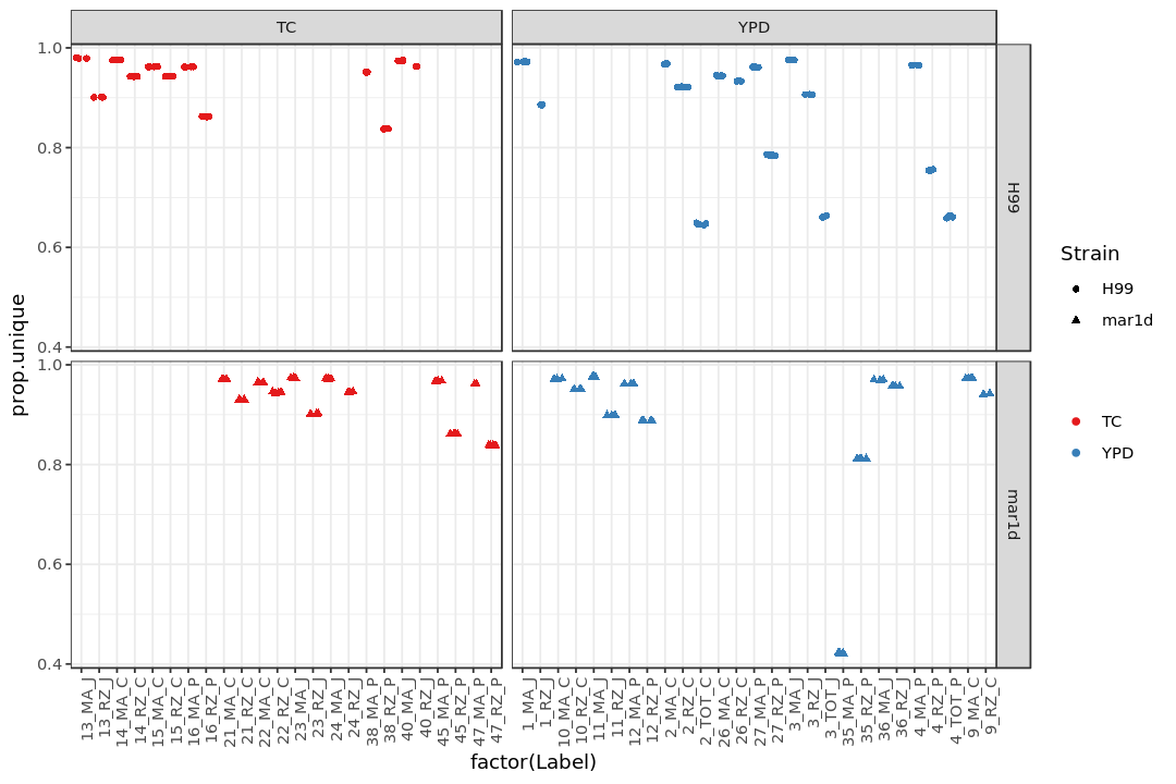
Show the fraction of unique mapped reads among all reads (prop.unique)¶

In [19]:

options(repr.plot.width = 9, repr.plot.height = 6)

p1 <- ggplot(annomapres,
             aes(x = factor(Label),
                 y = prop.unique,
                 shape = Strain,
                 color = Media)) +
        myfacet +
        mygeom +
        mytheme +
        mypal

print(p1)

../_images/pilot_02_Plot_Counts_33_0.png

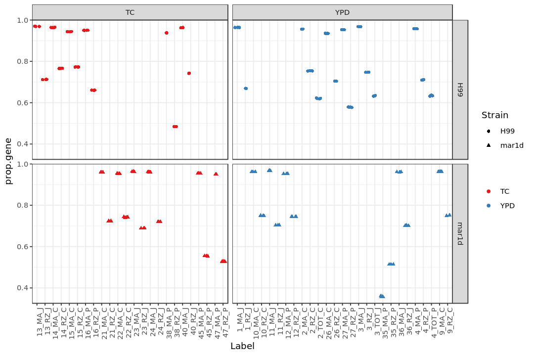
Show the fraction of reads mapped to genes (prop.gene)¶

In [20]:

options(repr.plot.width = 9, repr.plot.height = 6)

p2 <- ggplot(annomapres,
             aes(x = Label,
                 y = prop.gene,
                 shape = Strain,
                 color = Media)) +
        myfacet +
        mygeom +
        mytheme +
        mypal

print(p2)

../_images/pilot_02_Plot_Counts_35_0.png

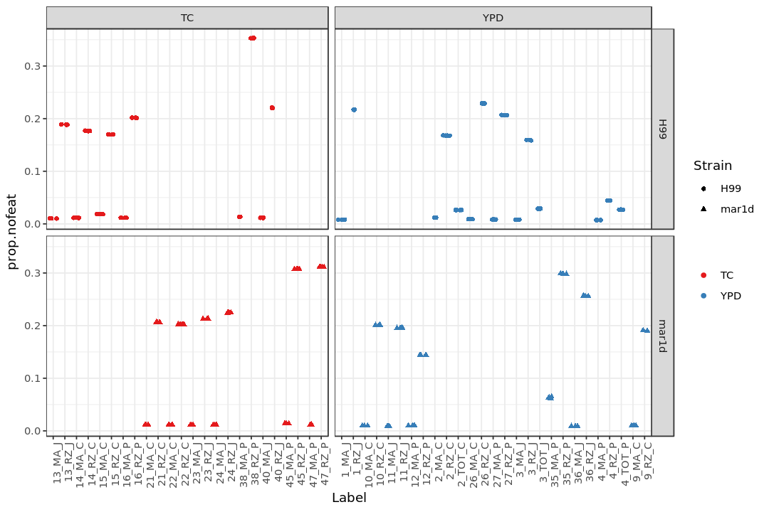
Show the fraction of reads categorized as “no feature” (prop.nofeat)¶

In [21]:

options(repr.plot.width = 9, repr.plot.height = 6)

p3 <- ggplot(annomapres,
             aes(x = Label,
                 y = prop.nofeat,
                 shape = Strain,
                 color = Media))+
        myfacet +
        mygeom +
        mytheme +
        mypal

print(p3)

../_images/pilot_02_Plot_Counts_37_0.png

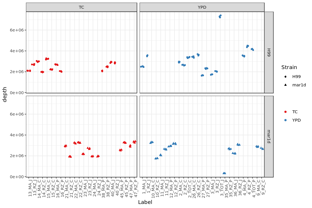
Show the number of all the reads in each sample¶

(Note: depth = ngenemap + namb + nmulti + nnofeat + nunmap)

In [22]:

options(repr.plot.width = 9, repr.plot.height = 6)

p4 <- ggplot(annomapres,
             aes(x = Label,
                 y = depth,
                 shape = Strain,
                 color = Media))+
        myfacet +
        mygeom +
        mytheme +
        mypal

print(p4)

../_images/pilot_02_Plot_Counts_39_0.png

Store the plots¶

In [23]:

png(file.path(IMGDIR, "p1.png"), height = 480 * 2, width = 480 * 2)
plot(p1)
graphics.off()

png(file.path(IMGDIR, "p2.png"), height = 480 * 2, width = 480 * 2)
plot(p2)
graphics.off()

png(file.path(IMGDIR, "p3.png"), height = 480 * 2, width = 480 * 2)
plot(p3)
graphics.off()

png(file.path(IMGDIR, "p4.png"), height = 480 * 2, width = 480 * 2)
plot(p4)
graphics.off()

The End¶

In [24]:

sessionInfo()

R version 3.4.1 (2017-06-30)
Platform: x86_64-pc-linux-gnu (64-bit)
Running under: Debian GNU/Linux 8 (jessie)

Matrix products: default
BLAS: /opt/conda/lib/R/lib/libRblas.so
LAPACK: /opt/conda/lib/R/lib/libRlapack.so

locale:
 [1] LC_CTYPE=en_US.UTF-8       LC_NUMERIC=C
 [3] LC_TIME=en_US.UTF-8        LC_COLLATE=en_US.UTF-8
 [5] LC_MONETARY=en_US.UTF-8    LC_MESSAGES=en_US.UTF-8
 [7] LC_PAPER=en_US.UTF-8       LC_NAME=C
 [9] LC_ADDRESS=C               LC_TELEPHONE=C
[11] LC_MEASUREMENT=en_US.UTF-8 LC_IDENTIFICATION=C

attached base packages:
 [1] tools     parallel  stats4    stats     graphics  grDevices utils
 [8] datasets  methods   base

other attached packages:
 [1] bindrcpp_0.2               plotly_4.8.0
 [3] dendextend_1.8.0           gridExtra_2.3
 [5] RColorBrewer_1.1-2         qvalue_2.10.0
 [7] limma_3.34.9               DESeq2_1.18.1
 [9] SummarizedExperiment_1.8.0 DelayedArray_0.4.1
[11] matrixStats_0.53.1         Biobase_2.38.0
[13] GenomicRanges_1.30.3       GenomeInfoDb_1.14.0
[15] IRanges_2.12.0             S4Vectors_0.16.0
[17] BiocGenerics_0.24.0        haven_1.1.1
[19] stringr_1.3.0              foreach_1.4.4
[21] dplyr_0.7.4                purrr_0.2.4
[23] readr_1.1.1                tidyr_0.8.1
[25] tibble_1.4.2               ggplot2_3.0.0
[27] tidyverse_1.1.1

loaded via a namespace (and not attached):
  [1] colorspace_1.3-2        class_7.3-14            modeltools_0.2-22
  [4] mclust_5.4.1            IRdisplay_0.4.4         htmlTable_1.9
  [7] XVector_0.18.0          base64enc_0.1-3         flexmix_2.3-14
 [10] bit64_0.9-5             mvtnorm_1.0-8           AnnotationDbi_1.40.0
 [13] lubridate_1.7.4         xml2_1.2.0              codetools_0.2-15
 [16] splines_3.4.1           mnormt_1.5-5            robustbase_0.92-7
 [19] geneplotter_1.56.0      knitr_1.20              IRkernel_0.8.11
 [22] Formula_1.2-1           jsonlite_1.5            broom_0.4.4
 [25] annotate_1.56.0         kernlab_0.9-25          cluster_2.0.6
 [28] compiler_3.4.1          httr_1.3.1              backports_1.1.2
 [31] assertthat_0.2.0        Matrix_1.2-14           lazyeval_0.2.1
 [34] acepack_1.4.1           htmltools_0.3.6         gtable_0.2.0
 [37] glue_1.2.0              GenomeInfoDbData_0.99.0 reshape2_1.4.3
 [40] Rcpp_0.12.15            trimcluster_0.1-2.1     cellranger_1.1.0
 [43] nlme_3.1-131            fpc_2.1-11.1            iterators_1.0.9
 [46] psych_1.8.4             rvest_0.3.2             XML_3.98-1.11
 [49] DEoptimR_1.0-8          MASS_7.3-48             zlibbioc_1.24.0
 [52] scales_0.5.0            hms_0.3                 memoise_1.1.0
 [55] rpart_4.1-13            latticeExtra_0.6-28     stringi_1.1.7
 [58] RSQLite_2.0             genefilter_1.60.0       checkmate_1.8.5
 [61] BiocParallel_1.12.0     repr_0.15.0             prabclus_2.2-6
 [64] rlang_0.2.1             pkgconfig_2.0.1         bitops_1.0-6
 [67] evaluate_0.10.1         lattice_0.20-34         bindr_0.1.1
 [70] labeling_0.3            htmlwidgets_1.2         tidyselect_0.2.4
 [73] bit_1.1-12              plyr_1.8.4              magrittr_1.5
 [76] R6_2.2.2                Hmisc_4.0-3             pbdZMQ_0.3-2
 [79] DBI_1.0.0               pillar_1.2.2            whisker_0.3-2
 [82] foreign_0.8-67          withr_2.1.1             survival_2.40-1
 [85] RCurl_1.95-4.8          nnet_7.3-12             modelr_0.1.2
 [88] crayon_1.3.4            uuid_0.1-2              viridis_0.5.1
 [91] locfit_1.5-9.1          grid_3.4.1              readxl_1.1.0
 [94] data.table_1.10.4       blob_1.1.1              forcats_0.3.0
 [97] diptest_0.75-7          digest_0.6.15           xtable_1.8-2
[100] munsell_0.5.0           viridisLite_0.3.0