Set environment¶

In [1]:

# load required libraries
library(DESeq2)
library(tidyverse)
library(RColorBrewer)
library(dendextend)

Loading required package: S4Vectors
Loading required package: stats4
Loading required package: BiocGenerics
Loading required package: parallel

Attaching package: ‘BiocGenerics’

The following objects are masked from ‘package:parallel’:

    clusterApply, clusterApplyLB, clusterCall, clusterEvalQ,
    clusterExport, clusterMap, parApply, parCapply, parLapply,
    parLapplyLB, parRapply, parSapply, parSapplyLB

The following objects are masked from ‘package:stats’:

    IQR, mad, sd, var, xtabs

The following objects are masked from ‘package:base’:

    anyDuplicated, append, as.data.frame, cbind, colMeans, colnames,
    colSums, do.call, duplicated, eval, evalq, Filter, Find, get, grep,
    grepl, intersect, is.unsorted, lapply, lengths, Map, mapply, match,
    mget, order, paste, pmax, pmax.int, pmin, pmin.int, Position, rank,
    rbind, Reduce, rowMeans, rownames, rowSums, sapply, setdiff, sort,
    table, tapply, union, unique, unsplit, which, which.max, which.min


Attaching package: ‘S4Vectors’

The following object is masked from ‘package:base’:

    expand.grid

Loading required package: IRanges
Loading required package: GenomicRanges
Loading required package: GenomeInfoDb
Loading required package: SummarizedExperiment
Loading required package: Biobase
Welcome to Bioconductor

    Vignettes contain introductory material; view with
    'browseVignettes()'. To cite Bioconductor, see
    'citation("Biobase")', and for packages 'citation("pkgname")'.

Loading required package: DelayedArray
Loading required package: matrixStats

Attaching package: ‘matrixStats’

The following objects are masked from ‘package:Biobase’:

    anyMissing, rowMedians


Attaching package: ‘DelayedArray’

The following objects are masked from ‘package:matrixStats’:

    colMaxs, colMins, colRanges, rowMaxs, rowMins, rowRanges

The following object is masked from ‘package:base’:

    apply

Loading tidyverse: ggplot2
Loading tidyverse: tibble
Loading tidyverse: tidyr
Loading tidyverse: readr
Loading tidyverse: purrr
Loading tidyverse: dplyr
Conflicts with tidy packages ---------------------------------------------------
collapse(): dplyr, IRanges
combine():  dplyr, Biobase, BiocGenerics
count():    dplyr, matrixStats
desc():     dplyr, IRanges
expand():   tidyr, S4Vectors
filter():   dplyr, stats
first():    dplyr, S4Vectors
lag():      dplyr, stats
Position(): ggplot2, BiocGenerics, base
reduce():   purrr, GenomicRanges, IRanges
rename():   dplyr, S4Vectors
slice():    dplyr, IRanges

---------------------
Welcome to dendextend version 1.8.0
Type citation('dendextend') for how to cite the package.

Type browseVignettes(package = 'dendextend') for the package vignette.
The github page is: https://github.com/talgalili/dendextend/

Suggestions and bug-reports can be submitted at: https://github.com/talgalili/dendextend/issues
Or contact: <tal.galili@gmail.com>

        To suppress this message use:  suppressPackageStartupMessages(library(dendextend))
---------------------


Attaching package: ‘dendextend’

The following object is masked from ‘package:stats’:

    cutree

Your Folder Structure:
└── HTS2018
    ├── out
    │   └── hts-pilot-2018.RData
    |   └── HTS-Pilot-Annotated-STAR-counts.RData
    └── img

In [3]:

# set directories
outdir <- "/home/jovyan/work/HTS2018/out"
imgdir <- "/home/jovyan/work/HTS2018/img"

Read in data¶

In [4]:

attach(file.path(outdir, "HTS-Pilot-Annotated-STAR-counts.RData"))

Annotated mapping results¶

In [5]:

head(annomapres0)

Label	Strain	Media	experiment_person	libprep_person	enrichment_method	prob.gene	prob.nofeat	prob.unique	depth
1_MA_J	H99	YPD	S	J	MA	0.9641456	0.008161923	0.9723075	2493464
1_RZ_J	H99	YPD	S	J	RZ	0.6689001	0.217095621	0.8859957	3541358
10_MA_C	mar1d	YPD	S	C	MA	0.9618651	0.009818573	0.9716837	3282785
10_RZ_C	mar1d	YPD	S	C	RZ	0.7497438	0.200651686	0.9503955	1742594
11_MA_J	mar1d	YPD	S	J	MA	0.9669597	0.008717898	0.9756776	2062181
11_RZ_J	mar1d	YPD	S	J	RZ	0.7030020	0.195547151	0.8985491	2621913

Annotated count matrix¶

In [6]:

head(annogenecnts0)

gene	1_MA_J	1_RZ_J	10_MA_C	10_RZ_C	11_MA_J	11_RZ_J	12_MA_P	12_RZ_P	13_MA_J	⋯	4_RZ_P	4_TOT_P	40_MA_J	40_RZ_J	45_MA_P	45_RZ_P	47_MA_P	47_RZ_P	9_MA_C	9_RZ_C
CNAG_00001	0	0	0	0	0	0	0	0	0	⋯	0	0	0	0	0	0	0	0	0	0
CNAG_00002	265	204	269	76	130	92	205	64	308	⋯	51	13	519	235	410	122	534	112	217	106
CNAG_00003	112	40	171	24	124	18	150	34	221	⋯	11	8	218	53	232	46	240	41	128	35
CNAG_00004	301	207	407	141	272	179	351	156	533	⋯	50	36	719	442	518	238	622	277	310	234
CNAG_00005	114	125	50	25	38	32	38	12	202	⋯	25	14	344	270	202	81	256	118	45	40
CNAG_00006	1904	1295	3571	1015	2073	1327	3003	926	1660	⋯	319	110	3002	1535	3934	1090	4966	1132	3313	1509

DESeq object¶

Generate count matrix for RZ enrichment method

In [7]:

### Prepare columnData (DataFrameand countData (matrix object)
### Select samples from RZ
annomapres0 %>%
    dplyr::filter(enrichment_method == "RZ")  %>%
    DataFrame ->
    columnData
rownames(columnData) <- columnData[["Label"]]

annogenecnts0 %>%
    dplyr::select(dput(as.character(c("gene",columnData[["Label"]])))) %>%
    as.data.frame %>%
    column_to_rownames("gene") %>%
    as.matrix ->
    countData

c("gene", "1_RZ_J", "10_RZ_C", "11_RZ_J", "12_RZ_P", "13_RZ_J",
"14_RZ_C", "15_RZ_C", "16_RZ_P", "2_RZ_C", "21_RZ_C", "22_RZ_C",
"23_RZ_J", "24_RZ_J", "26_RZ_C", "27_RZ_P", "3_RZ_J", "35_RZ_P",
"36_RZ_J", "38_RZ_P", "4_RZ_P", "40_RZ_J", "45_RZ_P", "47_RZ_P",
"9_RZ_C")

In [8]:

head(countData)

	1_RZ_J	10_RZ_C	11_RZ_J	12_RZ_P	13_RZ_J	14_RZ_C	15_RZ_C	16_RZ_P	2_RZ_C	21_RZ_C	⋯	27_RZ_P	3_RZ_J	35_RZ_P	36_RZ_J	38_RZ_P	4_RZ_P	40_RZ_J	45_RZ_P	47_RZ_P	9_RZ_C
CNAG_00001	0	0	0	0	0	0	0	1	0	0	⋯	0	0	0	0	0	0	0	0	0	0
CNAG_00002	204	76	92	64	230	182	200	129	168	124	⋯	43	107	150	109	95	51	235	122	112	106
CNAG_00003	40	24	18	34	56	53	54	40	40	41	⋯	9	24	26	43	43	11	53	46	41	35
CNAG_00004	207	141	179	156	396	363	416	254	184	312	⋯	56	140	224	202	166	50	442	238	277	234
CNAG_00005	125	25	32	12	201	179	187	124	121	122	⋯	22	67	154	56	82	25	270	81	118	40
CNAG_00006	1295	1015	1327	926	1143	879	1058	619	1060	1103	⋯	398	827	869	1877	627	319	1535	1090	1132	1509

Import count matrix as a DESeq object

In [9]:

### Make DESeq object on the basis of the counts
dds <- DESeqDataSetFromMatrix(countData, columnData, ~ Media + Strain + Media:Strain)
### Estimate Size Factors
dds <- estimateSizeFactors(dds)
### Estimate Dispersion parameters (for each gene)
dds <- estimateDispersions(dds)
### Fit NB MLE model
dds <- DESeq(dds)
### Rlog "normalized" expressions
rld <- rlog(dds)

gene-wise dispersion estimates
mean-dispersion relationship
final dispersion estimates
using pre-existing size factors
estimating dispersions
found already estimated dispersions, replacing these
gene-wise dispersion estimates
mean-dispersion relationship
final dispersion estimates
fitting model and testing

In [10]:

### Show top 10 hits
results(dds, tidy = TRUE) %>% arrange(pvalue) %>% head(10)

row	baseMean	log2FoldChange	lfcSE	stat	pvalue	padj
CNAG_04307	490.86196	4.023118	0.29759976	13.518553	1.215429e-41	9.552054e-38
CNAG_05459	636.02477	1.144042	0.09994094	11.447183	2.429119e-30	9.545224e-27
CNAG_03621	1821.27006	-1.064434	0.10659585	-9.985699	1.760551e-23	4.612056e-20
CNAG_00600	848.44047	1.142434	0.11598632	9.849729	6.872879e-23	1.350349e-19
CNAG_04585	812.31911	-4.040747	0.41261597	-9.792997	1.206656e-22	1.896623e-19
CNAG_03735	521.96604	1.634231	0.16755798	9.753228	1.786944e-22	2.340599e-19
CNAG_07862	85.91321	-2.608844	0.26841617	-9.719401	2.492446e-22	2.798304e-19
CNAG_02733	15.32034	-4.023640	0.41731949	-9.641629	5.333480e-22	5.239478e-19
CNAG_06517	850.38128	1.871991	0.19539060	9.580764	9.632973e-22	8.411726e-19
CNAG_00399	213.68536	-2.146601	0.22469243	-9.553507	1.253786e-21	9.853503e-19

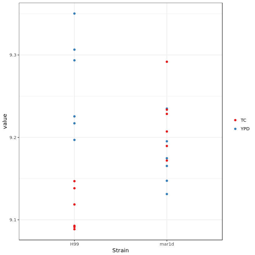
Gene expression value in different media and strain¶

In [11]:

### A function for exploring interactions
myinteractplot <- function(mydds, geneid) {
    # plot gene expression value in different media and strain
    #
    # Args:
    #   mydds (DESeqTransform object): your input DESeq object
    #   geneid (Charater): the second count data
    #
    # Returns:
    #   (ggplot object) the final plot
    assay(mydds) %>%
        as_tibble(rownames = "gene") %>%
        filter(gene == geneid) %>%
        gather(Label, value, -gene) %>%
        select(-gene) ->
        genedat

    colData(mydds) %>%
        as.data.frame %>%
        as_tibble %>%
        full_join(genedat, by="Label") -> genedat

    mygeom  <-  geom_point()
    mypal   <- scale_colour_manual(name = "",  values = brewer.pal(3, "Set1"))
    mytheme <- theme_bw()

    ggplot(genedat, aes(x = Strain, y = value, color = Media)) + mygeom + mytheme + mypal
}

myinteractplot(rld, "CNAG_05845")

Data type cannot be displayed:

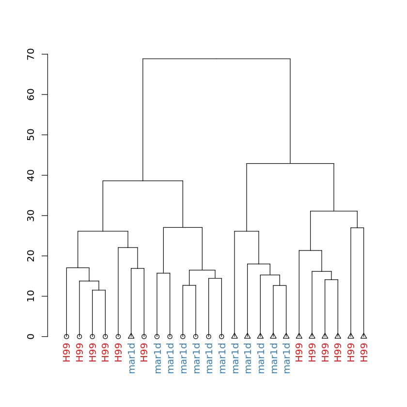
../_images/pilot_03_Compare_Gene_Expression_18_1.png

Dendrogram of Samples in Hierarchical Clustering¶

Create Dendrogram of samples using hierarchical clustering

In [12]:

assay(rld) %>%
    t() %>%
    dist %>%
    hclust(method = "complete") %>%
    as.dendrogram ->
    mydend

Customize function to plot dendrogram showing the sample annotations

In [13]:

dendplot <- function(mydend, columndata, labvar, colvar, pchvar) {
    # plot dendrogram
    #
    # Args:
    #   mydend (Dendrogram): your input DESeq object
    #   columndata (DataFrame): the second count data
    #   labvar (Character): variable that show in label
    #   colvar (Character): variable that define color
    #   pchvar (Character): variable that define shape of points
    #
    # Returns:
    #   (Dendrogram) final plot of dendrogram
    cols   <- factor(columndata[[colvar]][order.dendrogram(mydend)])
    collab <- brewer.pal(max(3, nlevels(cols)), "Set1")[cols]
    pchs   <- factor(columndata[[pchvar]][order.dendrogram(mydend)])
    pchlab <- seq_len(nlevels(pchs))[pchs]
    lablab <- columndata[[labvar]][order.dendrogram(mydend)]

    mydend %>%
        set("labels_cex", 1) %>%
        set("labels_col", collab) %>%
        set("leaves_pch", pchlab) %>%
        set("labels",     lablab)
}

Dendrogram of samples: showing strain of each sample¶

In [14]:

dendplot(mydend, columnData, "Strain", "Strain", "Media") %>% plot

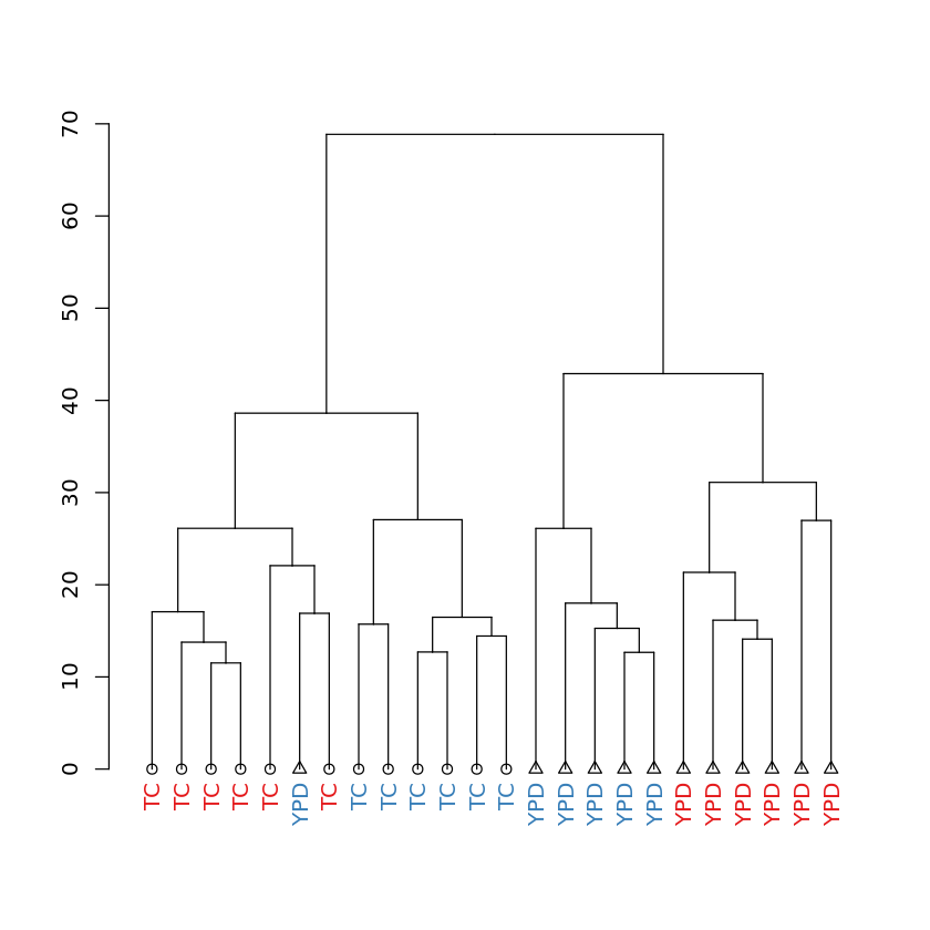
../_images/pilot_03_Compare_Gene_Expression_25_0.png

Dendrogram of samples: showing media of each sample¶

In [15]:

dendplot(mydend, columnData, "Media", "Strain", "Media") %>% plot

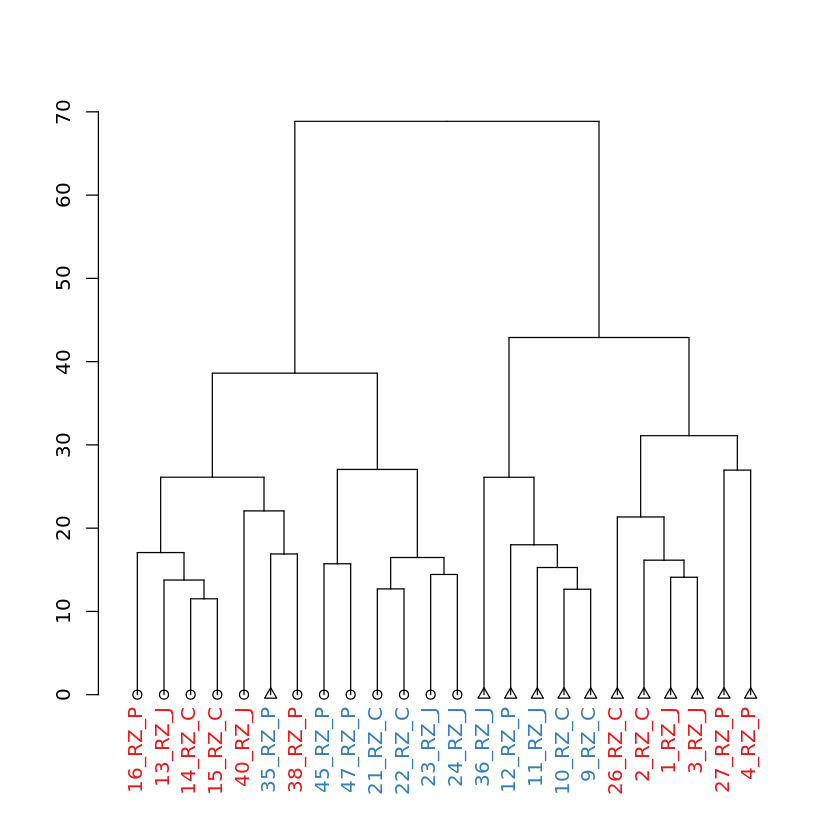
../_images/pilot_03_Compare_Gene_Expression_27_0.png

Dendrogram of samples: showing sample names of each sample¶

In [16]:

dendplot(mydend, columnData, "Label", "Strain", "Media") %>% plot

../_images/pilot_03_Compare_Gene_Expression_29_0.png

Store the plot into a pdf

In [17]:

pdf(file.path(imgdir, "dendrogram.pdf"))
dendplot(mydend, columnData, "Strain", "Strain", "Media") %>% plot
dendplot(mydend, columnData, "Media", "Strain", "Media") %>% plot
dendplot(mydend, columnData, "Label", "Strain", "Media") %>% plot
graphics.off()