[1]:
%matplotlib inline
import networkx as nx
from networkx.drawing.nx_pydot import graphviz_layout
from networkx.drawing.layout import planar_layout
import matplotlib.pyplot as plt
from matplotlib.colors import LinearSegmentedColormap
import pandas as pd
import numpy as np
Graph concepts
elements
graph
vertex
edge
path
graph properties
directed or undirected
weighted or unweighted
cyclic or acyclic
single or multiple edges
connected or disconnected
vertex properties
in-degree
out-degree
centrality
edge properties
direction
weight
multiplicity
Graph representations
Vertex and edge collections
Adjacency list
Adjacency matrix
Sparse matrix
[2]:
%matplotlib inline
import networkx as nx
from pprint import pprint
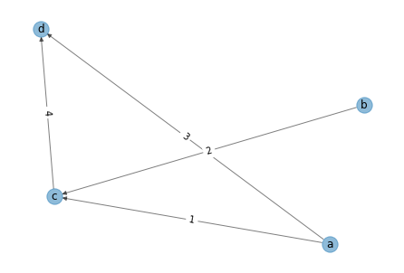
[3]:
vs = ['a', 'b', 'c', 'd']
es = [('a','c', 1), ('b','c', 2), ('a','d', 3), ('c', 'd', 4)]

g1 = nx.DiGraph()
g1.add_nodes_from(vs)
g1.add_weighted_edges_from(es)

pos = nx.spring_layout(g1)
labels = nx.get_edge_attributes(g1,'weight')
nx.draw(g1, pos=pos, alpha=0.5)
nx.draw_networkx_edge_labels(g1, pos=pos, edge_labels=labels)
nx.draw_networkx_labels(g1, pos=pos)
pass
[4]:
import sys
[5]:
nx.write_adjlist(g1, sys.stdout)
#/usr/local/lib/python3.8/site-packages/ipykernel_launcher.py -f /Users/cliburnchan/Library/Jupyter/runtime/kernel-cbc7a826-65d9-4be6-993f-cecdb1c227ba.json
# GMT Thu Nov 12 00:34:55 2020
#
a c d
b c
c d
d
[6]:
print(nx.adj_matrix(g1))
  (0, 2)        1
  (0, 3)        3
  (1, 2)        2
  (2, 3)        4
[7]:
nx.adj_matrix(g1).todense()
[7]:
matrix([[0, 0, 1, 3],
        [0, 0, 2, 0],
        [0, 0, 0, 4],
        [0, 0, 0, 0]])
[8]:
#### Standard format for graph exchange is GraphML
[9]:
nx.write_gml(g1, sys.stdout)
graph [
  directed 1
  node [
    id 0
    label "a"
  ]
  node [
    id 1
    label "b"
  ]
  node [
    id 2
    label "c"
  ]
  node [
    id 3
    label "d"
  ]
  edge [
    source 0
    target 2
    weight 1
  ]
  edge [
    source 0
    target 3
    weight 3
  ]
  edge [
    source 1
    target 2
    weight 2
  ]
  edge [
    source 2
    target 3
    weight 4
  ]
]
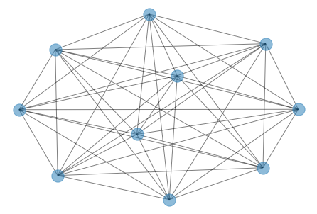
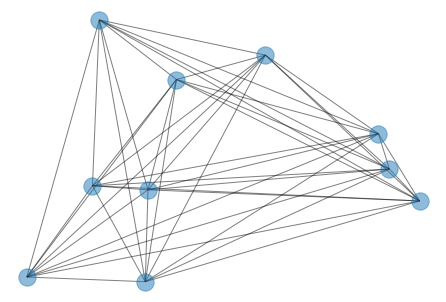
Some examples
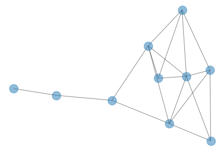
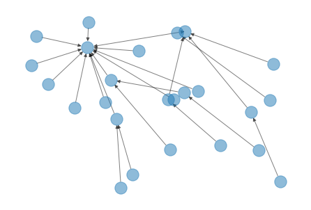
[10]:
n = 50
k = 6
p =0.3
g = nx.watts_strogatz_graph(n, k, p)

Graph Algorithms
[16]:
! python3 -m pip install --quiet pydot python-louvain
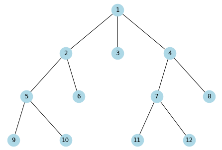
Search
[17]:
g = {
    1: [2,3,4],
    2: [5,6],
    3: [],
    4: [7,8],
    5: [9,10],
    6: [],
    7: [11, 12],
    8: [],
    9: [],
    10: [],
    11: [],
    12: []
}
[18]:
G = nx.from_dict_of_lists(g)
[19]:
pos = graphviz_layout(G, prog='dot')
[20]:
nx.draw(G, pos, with_labels=True, node_size=600, node_color='lightblue')
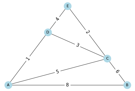
Pathfinding
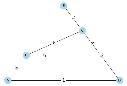
[23]:
edges = [
    ('A', 'B', 8),
    ('A', 'C', 5),
    ('A', 'D', 1),
    ('B', 'C', 6),
    ('C', 'D', 3),
    ('C', 'E', 2),
    ('D', 'E', 4)
]
[24]:
G = nx.Graph()
G.add_weighted_edges_from(edges)
[25]:
pos = planar_layout(G)
nx.draw(G,
        pos,
        with_labels=True,
        node_size=600,
        node_color='lightblue')
labels = nx.draw_networkx_edge_labels(
    G,
    pos,
    edge_labels={(x[0], x[1]): str(x[2]) for x in edges},
    font_size=15,
)
Single source shortest path
[27]:
list(nx.single_source_dijkstra(G, 'A'))
[27]:
[{'A': 0, 'D': 1, 'C': 4, 'E': 5, 'B': 8},
 {'A': ['A'],
  'B': ['A', 'B'],
  'C': ['A', 'D', 'C'],
  'D': ['A', 'D'],
  'E': ['A', 'D', 'E']}]
All pairs shortest path
[28]:
list(nx.all_pairs_dijkstra_path(G))
[28]:
[('A',
  {'A': ['A'],
   'B': ['A', 'B'],
   'C': ['A', 'D', 'C'],
   'D': ['A', 'D'],
   'E': ['A', 'D', 'E']}),
 ('B',
  {'B': ['B'],
   'A': ['B', 'A'],
   'C': ['B', 'C'],
   'D': ['B', 'C', 'D'],
   'E': ['B', 'C', 'E']}),
 ('C',
  {'C': ['C'],
   'A': ['C', 'D', 'A'],
   'B': ['C', 'B'],
   'D': ['C', 'D'],
   'E': ['C', 'E']}),
 ('D',
  {'D': ['D'],
   'A': ['D', 'A'],
   'C': ['D', 'C'],
   'E': ['D', 'E'],
   'B': ['D', 'A', 'B']}),
 ('E',
  {'E': ['E'],
   'C': ['E', 'C'],
   'D': ['E', 'D'],
   'A': ['E', 'D', 'A'],
   'B': ['E', 'C', 'B']})]
Minimal spanning tree
[29]:
G_min = nx.minimum_spanning_tree(G)
[30]:
pos = planar_layout(G_min)
nx.draw(G_min,
        pos,
        with_labels=True,
        node_size=600,
        node_color='lightblue')
labels = nx.draw_networkx_edge_labels(
    G_min,
    pos,
    edge_labels={(x[0], x[1]): str(x[2]) for x in edges},
    font_size=15,
)
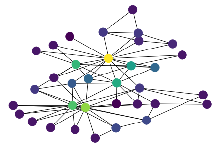
Centrality
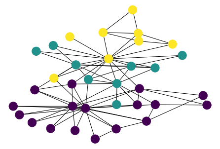
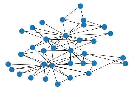
[31]:
G = nx.karate_club_graph()
[32]:
pos = nx.kamada_kawai_layout(G)
[33]:
nx.draw(G, pos)
[34]:
plt.viridis()
<Figure size 432x288 with 0 Axes>
[35]:
values = nx.degree(G)
n_color = np.asarray([values(n) for n in G.nodes()])
nx.draw(G, pos, node_color=n_color)
[36]:
help(nx.closeness_centrality)
Help on function closeness_centrality in module networkx.algorithms.centrality.closeness:

closeness_centrality(G, u=None, distance=None, wf_improved=True)
    Compute closeness centrality for nodes.

    Closeness centrality [1]_ of a node `u` is the reciprocal of the
    average shortest path distance to `u` over all `n-1` reachable nodes.

    .. math::

        C(u) = \frac{n - 1}{\sum_{v=1}^{n-1} d(v, u)},

    where `d(v, u)` is the shortest-path distance between `v` and `u`,
    and `n` is the number of nodes that can reach `u`. Notice that the
    closeness distance function computes the incoming distance to `u`
    for directed graphs. To use outward distance, act on `G.reverse()`.

    Notice that higher values of closeness indicate higher centrality.

    Wasserman and Faust propose an improved formula for graphs with
    more than one connected component. The result is "a ratio of the
    fraction of actors in the group who are reachable, to the average
    distance" from the reachable actors [2]_. You might think this
    scale factor is inverted but it is not. As is, nodes from small
    components receive a smaller closeness value. Letting `N` denote
    the number of nodes in the graph,

    .. math::

        C_{WF}(u) = \frac{n-1}{N-1} \frac{n - 1}{\sum_{v=1}^{n-1} d(v, u)},

    Parameters
    ----------
    G : graph
      A NetworkX graph

    u : node, optional
      Return only the value for node u

    distance : edge attribute key, optional (default=None)
      Use the specified edge attribute as the edge distance in shortest
      path calculations

    wf_improved : bool, optional (default=True)
      If True, scale by the fraction of nodes reachable. This gives the
      Wasserman and Faust improved formula. For single component graphs
      it is the same as the original formula.

    Returns
    -------
    nodes : dictionary
      Dictionary of nodes with closeness centrality as the value.

    See Also
    --------
    betweenness_centrality, load_centrality, eigenvector_centrality,
    degree_centrality, incremental_closeness_centrality

    Notes
    -----
    The closeness centrality is normalized to `(n-1)/(|G|-1)` where
    `n` is the number of nodes in the connected part of graph
    containing the node.  If the graph is not completely connected,
    this algorithm computes the closeness centrality for each
    connected part separately scaled by that parts size.

    If the 'distance' keyword is set to an edge attribute key then the
    shortest-path length will be computed using Dijkstra's algorithm with
    that edge attribute as the edge weight.

    The closeness centrality uses *inward* distance to a node, not outward.
    If you want to use outword distances apply the function to `G.reverse()`

    In NetworkX 2.2 and earlier a bug caused Dijkstra's algorithm to use the
    outward distance rather than the inward distance. If you use a 'distance'
    keyword and a DiGraph, your results will change between v2.2 and v2.3.

    References
    ----------
    .. [1] Linton C. Freeman: Centrality in networks: I.
       Conceptual clarification. Social Networks 1:215-239, 1979.
       http://leonidzhukov.ru/hse/2013/socialnetworks/papers/freeman79-centrality.pdf
    .. [2] pg. 201 of Wasserman, S. and Faust, K.,
       Social Network Analysis: Methods and Applications, 1994,
       Cambridge University Press.
[37]:
values = nx.closeness_centrality(G)
n_color = np.asarray([values[n] for n in G.nodes()])
nx.draw(G, pos, node_color=n_color)

[38]:
help(nx.pagerank)
Help on function pagerank in module networkx.algorithms.link_analysis.pagerank_alg:

pagerank(G, alpha=0.85, personalization=None, max_iter=100, tol=1e-06, nstart=None, weight='weight', dangling=None)
    Returns the PageRank of the nodes in the graph.

    PageRank computes a ranking of the nodes in the graph G based on
    the structure of the incoming links. It was originally designed as
    an algorithm to rank web pages.

    Parameters
    ----------
    G : graph
      A NetworkX graph.  Undirected graphs will be converted to a directed
      graph with two directed edges for each undirected edge.

    alpha : float, optional
      Damping parameter for PageRank, default=0.85.

    personalization: dict, optional
      The "personalization vector" consisting of a dictionary with a
      key some subset of graph nodes and personalization value each of those.
      At least one personalization value must be non-zero.
      If not specfiied, a nodes personalization value will be zero.
      By default, a uniform distribution is used.

    max_iter : integer, optional
      Maximum number of iterations in power method eigenvalue solver.

    tol : float, optional
      Error tolerance used to check convergence in power method solver.

    nstart : dictionary, optional
      Starting value of PageRank iteration for each node.

    weight : key, optional
      Edge data key to use as weight.  If None weights are set to 1.

    dangling: dict, optional
      The outedges to be assigned to any "dangling" nodes, i.e., nodes without
      any outedges. The dict key is the node the outedge points to and the dict
      value is the weight of that outedge. By default, dangling nodes are given
      outedges according to the personalization vector (uniform if not
      specified). This must be selected to result in an irreducible transition
      matrix (see notes under google_matrix). It may be common to have the
      dangling dict to be the same as the personalization dict.

    Returns
    -------
    pagerank : dictionary
       Dictionary of nodes with PageRank as value

    Examples
    --------
    >>> G = nx.DiGraph(nx.path_graph(4))
    >>> pr = nx.pagerank(G, alpha=0.9)

    Notes
    -----
    The eigenvector calculation is done by the power iteration method
    and has no guarantee of convergence.  The iteration will stop after
    an error tolerance of ``len(G) * tol`` has been reached. If the
    number of iterations exceed `max_iter`, a
    :exc:`networkx.exception.PowerIterationFailedConvergence` exception
    is raised.

    The PageRank algorithm was designed for directed graphs but this
    algorithm does not check if the input graph is directed and will
    execute on undirected graphs by converting each edge in the
    directed graph to two edges.

    See Also
    --------
    pagerank_numpy, pagerank_scipy, google_matrix

    Raises
    ------
    PowerIterationFailedConvergence
        If the algorithm fails to converge to the specified tolerance
        within the specified number of iterations of the power iteration
        method.

    References
    ----------
    .. [1] A. Langville and C. Meyer,
       "A survey of eigenvector methods of web information retrieval."
       http://citeseer.ist.psu.edu/713792.html
    .. [2] Page, Lawrence; Brin, Sergey; Motwani, Rajeev and Winograd, Terry,
       The PageRank citation ranking: Bringing order to the Web. 1999
       http://dbpubs.stanford.edu:8090/pub/showDoc.Fulltext?lang=en&doc=1999-66&format=pdf
[39]:
values = nx.pagerank(G)
n_color = np.asarray([values[n] for n in G.nodes()])
nx.draw(G, pos, node_color=n_color)
Community Detection
Triangles
[40]:
help(nx.triangles)
Help on function triangles in module networkx.algorithms.cluster:

triangles(G, nodes=None)
    Compute the number of triangles.

    Finds the number of triangles that include a node as one vertex.

    Parameters
    ----------
    G : graph
       A networkx graph
    nodes : container of nodes, optional (default= all nodes in G)
       Compute triangles for nodes in this container.

    Returns
    -------
    out : dictionary
       Number of triangles keyed by node label.

    Examples
    --------
    >>> G = nx.complete_graph(5)
    >>> print(nx.triangles(G, 0))
    6
    >>> print(nx.triangles(G))
    {0: 6, 1: 6, 2: 6, 3: 6, 4: 6}
    >>> print(list(nx.triangles(G, (0, 1)).values()))
    [6, 6]

    Notes
    -----
    When computing triangles for the entire graph each triangle is counted
    three times, once at each node.  Self loops are ignored.
[41]:
values = nx.triangles(G)
n_color = np.asarray([values[n] for n in G.nodes()])
nx.draw(G, pos, node_color=n_color)
Clustering coefficient
[42]:
help(nx.clustering)
Help on function clustering in module networkx.algorithms.cluster:

clustering(G, nodes=None, weight=None)
    Compute the clustering coefficient for nodes.

    For unweighted graphs, the clustering of a node :math:`u`
    is the fraction of possible triangles through that node that exist,

    .. math::

      c_u = \frac{2 T(u)}{deg(u)(deg(u)-1)},

    where :math:`T(u)` is the number of triangles through node :math:`u` and
    :math:`deg(u)` is the degree of :math:`u`.

    For weighted graphs, there are several ways to define clustering [1]_.
    the one used here is defined
    as the geometric average of the subgraph edge weights [2]_,

    .. math::

       c_u = \frac{1}{deg(u)(deg(u)-1))}
             \sum_{vw} (\hat{w}_{uv} \hat{w}_{uw} \hat{w}_{vw})^{1/3}.

    The edge weights :math:`\hat{w}_{uv}` are normalized by the maximum weight
    in the network :math:`\hat{w}_{uv} = w_{uv}/\max(w)`.

    The value of :math:`c_u` is assigned to 0 if :math:`deg(u) < 2`.

    For directed graphs, the clustering is similarly defined as the fraction
    of all possible directed triangles or geometric average of the subgraph
    edge weights for unweighted and weighted directed graph respectively [3]_.

    .. math::

       c_u = \frac{1}{deg^{tot}(u)(deg^{tot}(u)-1) - 2deg^{\leftrightarrow}(u)}
             T(u),

    where :math:`T(u)` is the number of directed triangles through node
    :math:`u`, :math:`deg^{tot}(u)` is the sum of in degree and out degree of
    :math:`u` and :math:`deg^{\leftrightarrow}(u)` is the reciprocal degree of
    :math:`u`.

    Parameters
    ----------
    G : graph

    nodes : container of nodes, optional (default=all nodes in G)
       Compute clustering for nodes in this container.

    weight : string or None, optional (default=None)
       The edge attribute that holds the numerical value used as a weight.
       If None, then each edge has weight 1.

    Returns
    -------
    out : float, or dictionary
       Clustering coefficient at specified nodes

    Examples
    --------
    >>> G = nx.complete_graph(5)
    >>> print(nx.clustering(G, 0))
    1.0
    >>> print(nx.clustering(G))
    {0: 1.0, 1: 1.0, 2: 1.0, 3: 1.0, 4: 1.0}

    Notes
    -----
    Self loops are ignored.

    References
    ----------
    .. [1] Generalizations of the clustering coefficient to weighted
       complex networks by J. Saramäki, M. Kivelä, J.-P. Onnela,
       K. Kaski, and J. Kertész, Physical Review E, 75 027105 (2007).
       http://jponnela.com/web_documents/a9.pdf
    .. [2] Intensity and coherence of motifs in weighted complex
       networks by J. P. Onnela, J. Saramäki, J. Kertész, and K. Kaski,
       Physical Review E, 71(6), 065103 (2005).
    .. [3] Clustering in complex directed networks by G. Fagiolo,
       Physical Review E, 76(2), 026107 (2007).
[43]:
values = nx.clustering(G)
n_color = np.asarray([values[n] for n in G.nodes()])
nx.draw(G, pos, node_color=n_color)
[44]:
import matplotlib.colors as mcolors
[45]:
colors = list(mcolors.BASE_COLORS.keys())
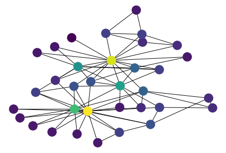
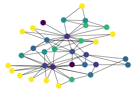
Label propagation
[46]:
help(nx.community.label_propagation_communities)
Help on function label_propagation_communities in module networkx.algorithms.community.label_propagation:

label_propagation_communities(G)
    Generates community sets determined by label propagation

    Finds communities in `G` using a semi-synchronous label propagation
    method[1]_. This method combines the advantages of both the synchronous
    and asynchronous models. Not implemented for directed graphs.

    Parameters
    ----------
    G : graph
        An undirected NetworkX graph.

    Yields
    ------
    communities : generator
        Yields sets of the nodes in each community.

    Raises
    ------
    NetworkXNotImplemented
       If the graph is directed

    References
    ----------
    .. [1] Cordasco, G., & Gargano, L. (2010, December). Community detection
       via semi-synchronous label propagation algorithms. In Business
       Applications of Social Network Analysis (BASNA), 2010 IEEE International
       Workshop on (pp. 1-8). IEEE.
[47]:
parts = list(nx.community.label_propagation_communities(G))
values = {n: i for i, ns in enumerate(parts) for n in ns}
n_color = np.asarray([values[n] for n in G.nodes()])
nx.draw(G, pos, node_color=n_color)
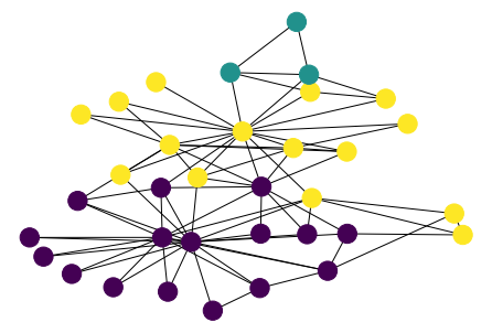
Clauset-Newman-Moore greedy modularity
Definition - Modularity is the fraction of the edges that fall within the given groups minus the expected fraction if edges were distributed at random.
[48]:
help(nx.community.greedy_modularity_communities)
Help on function greedy_modularity_communities in module networkx.algorithms.community.modularity_max:

greedy_modularity_communities(G, weight=None)
    Find communities in graph using Clauset-Newman-Moore greedy modularity
    maximization. This method currently supports the Graph class and does not
    consider edge weights.

    Greedy modularity maximization begins with each node in its own community
    and joins the pair of communities that most increases modularity until no
    such pair exists.

    Parameters
    ----------
    G : NetworkX graph

    Returns
    -------
    Yields sets of nodes, one for each community.

    Examples
    --------
    >>> from networkx.algorithms.community import greedy_modularity_communities
    >>> G = nx.karate_club_graph()
    >>> c = list(greedy_modularity_communities(G))
    >>> sorted(c[0])
    [8, 14, 15, 18, 20, 22, 23, 24, 25, 26, 27, 28, 29, 30, 31, 32, 33]

    References
    ----------
    .. [1] M. E. J Newman 'Networks: An Introduction', page 224
       Oxford University Press 2011.
    .. [2] Clauset, A., Newman, M. E., & Moore, C.
       "Finding community structure in very large networks."
       Physical Review E 70(6), 2004.
[49]:
parts = list(nx.community.greedy_modularity_communities(G))
values = {n: i for i, ns in enumerate(parts) for n in ns}
n_color = np.asarray([values[n] for n in G.nodes()])
nx.draw(G, pos, node_color=n_color)

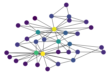
Louvain
This works well on large graphs, and is used to cluster single-cell RNA-seq data into cell subsets.
[50]:
import community as community_louvain
[51]:
help(community_louvain.best_partition)
Help on function best_partition in module community.community_louvain:

best_partition(graph, partition=None, weight='weight', resolution=1.0, randomize=None, random_state=None)
    Compute the partition of the graph nodes which maximises the modularity
    (or try..) using the Louvain heuristices

    This is the partition of highest modularity, i.e. the highest partition
    of the dendrogram generated by the Louvain algorithm.

    Parameters
    ----------
    graph : networkx.Graph
       the networkx graph which is decomposed
    partition : dict, optional
       the algorithm will start using this partition of the nodes.
       It's a dictionary where keys are their nodes and values the communities
    weight : str, optional
        the key in graph to use as weight. Default to 'weight'
    resolution :  double, optional
        Will change the size of the communities, default to 1.
        represents the time described in
        "Laplacian Dynamics and Multiscale Modular Structure in Networks",
        R. Lambiotte, J.-C. Delvenne, M. Barahona
    randomize : boolean, optional
        Will randomize the node evaluation order and the community evaluation
        order to get different partitions at each call
    random_state : int, RandomState instance or None, optional (default=None)
        If int, random_state is the seed used by the random number generator;
        If RandomState instance, random_state is the random number generator;
        If None, the random number generator is the RandomState instance used
        by `np.random`.

    Returns
    -------
    partition : dictionnary
       The partition, with communities numbered from 0 to number of communities

    Raises
    ------
    NetworkXError
       If the graph is not Eulerian.

    See Also
    --------
    generate_dendrogram to obtain all the decompositions levels

    Notes
    -----
    Uses Louvain algorithm

    References
    ----------
    .. 1. Blondel, V.D. et al. Fast unfolding of communities in
    large networks. J. Stat. Mech 10008, 1-12(2008).

    Examples
    --------
    >>>  #Basic usage
    >>> G=nx.erdos_renyi_graph(100, 0.01)
    >>> part = best_partition(G)

    >>> #other example to display a graph with its community :
    >>> #better with karate_graph() as defined in networkx examples
    >>> #erdos renyi don't have true community structure
    >>> G = nx.erdos_renyi_graph(30, 0.05)
    >>> #first compute the best partition
    >>> partition = community.best_partition(G)
    >>>  #drawing
    >>> size = float(len(set(partition.values())))
    >>> pos = nx.spring_layout(G)
    >>> count = 0.
    >>> for com in set(partition.values()) :
    >>>     count += 1.
    >>>     list_nodes = [nodes for nodes in partition.keys()
    >>>                                 if partition[nodes] == com]
    >>>     nx.draw_networkx_nodes(G, pos, list_nodes, node_size = 20,
                                    node_color = str(count / size))
    >>> nx.draw_networkx_edges(G, pos, alpha=0.5)
    >>> plt.show()
[52]:
partion = community_louvain.best_partition(G)
values = {n: i for i, ns in enumerate(parts) for n in ns}
n_color = np.asarray([values[n] for n in G.nodes()])
nx.draw(G, pos, node_color=n_color)