Hyperparameter tuning¶

There are 4 basic steps to hyperparameter tuning

Define the objective function
Define the space of hyperparameters to sample from
Define the metrics to optimize on
Run an optimization algorithm

The two simplest optimization algorithms are brute force search (aka Grid Search) and random sampling from the parameter space. Of course there are also more sophisticated search methods.

There are packages that provide wrappers for sklearn models and automatically use the model’s objective function, making the automation of tuning such models quite easy.

In practice, optimization is usually done over multiple model families - for simplicity we show only one model family but it is easy to find examples online.

[1]:

import numpy as np
import pandas as pd
import matplotlib.pyplot as plt

Load data¶

We use squeeze to convert a single column DataFrame to a Series.

[2]:

X_train = pd.read_csv('data/X_train.csv')
X_test = pd.read_csv('data/X_test.csv')
y_train = pd.read_csv('data/y_train.csv').squeeze()
y_test = pd.read_csv('data/y_test.csv').squeeze()

Using `skelearn`¶

[3]:

from sklearn.ensemble import RandomForestClassifier

[4]:

RandomForestClassifier().get_params().keys()

[4]:

dict_keys(['bootstrap', 'ccp_alpha', 'class_weight', 'criterion', 'max_depth', 'max_features', 'max_leaf_nodes', 'max_samples', 'min_impurity_decrease', 'min_impurity_split', 'min_samples_leaf', 'min_samples_split', 'min_weight_fraction_leaf', 'n_estimators', 'n_jobs', 'oob_score', 'random_state', 'verbose', 'warm_start'])

You can run

help(RandomForestClassifier)

to get more information about the parameters.

For optimization, you need to understand the ML algorithm and what each tuning parameter does, and also to have some idea of what is a sensible range of values for each parameter. If in doubt, some orders of magnitude below and above the default value is a simple heuristic. In this example, we will tune the following (sklearn defaults in parentheses):

criterion = measure used to determine whether to split (Gini)
n_estimators = n of trees (100)
max_features = max number of features considered for splitting a node (sqrt(n_features)
max_depth = max number of levels in each decision tree (None)
min_samples_split = min number of data points placed in a node before the node is split (2)
min_samples_leaf = min number of data points allowed in a leaf node (1)

We will search over the following

criterion Gini, entropy
n_estimators 50, 100, 200
max_features 0.1, 0.3, 0.5, sqrt, log
max_depth 1, 3, 5, 10, None
min_samples_split 2, 5, 10
min_samples_leaf 1, 2, 5, 10

[5]:

from sklearn.model_selection import (
    RandomizedSearchCV,
    GridSearchCV
)

[6]:

params1 = {
    'criterion': ['gini', 'entropy'],
    'n_estimators': [50, 100, 200],
    'max_features': [0.1, 0.3, 0.5, 'sqrt', 'log'],
    'max_depth': [1, 3, 5, 10, None],
    'min_samples_split': [2, 5, 10],
    'min_samples_leaf': [1, 2, 5, 10],
}

This looks simple enough, but there are 1800 combinations to search!

[7]:

np.prod(list(map(len, params1.values())))

[7]:

[8]:

rf = RandomForestClassifier()

Grid Search¶

[9]:

%%time
clf_gs = GridSearchCV(
    rf,
    params1,
    n_jobs=-1,
).fit(X_train, y_train)

CPU times: user 20.9 s, sys: 1.79 s, total: 22.7 s
Wall time: 4min 44s

For other searchers, we limit to 32 trials simply to save time. In practice, you could use a larger number for a more comprehensive search.

[10]:

N = 32

Randomized Search¶

This is similar but searches a random subset of the specified parameters.

[11]:

%%time
clf_rs1 = RandomizedSearchCV(
    rf,
    params1,
    n_jobs=-1,
    random_state=0,
    n_iter=N,
).fit(X_train, y_train)

CPU times: user 462 ms, sys: 20.9 ms, total: 482 ms
Wall time: 5.16 s

Using parameter distributions¶

[12]:

from scipy.stats import randint, uniform

[13]:

params2 = {
    'criterion': ['gini', 'entropy'],
    'n_estimators': randint(50, 201),
    'max_features': uniform(0, 1),
    'max_depth': randint(1, 101),
    'min_samples_split': randint(2, 11),
    'min_samples_leaf': randint(1, 11),
}

[14]:

%%time
clf_rs2 = RandomizedSearchCV(
    rf,
    params2,
    n_jobs=-1,
    random_state=0,
    n_iter=N,
).fit(X_train, y_train)

CPU times: user 671 ms, sys: 34.4 ms, total: 705 ms
Wall time: 7.62 s

Using `scikit-otpimize`¶

[15]:

! python3 -m pip install --quiet scikit-optimize

[16]:

from skopt import BayesSearchCV
from skopt.space import Real, Categorical, Integer

[17]:

p = X_train.shape[1]

[18]:

params3 = {
    'criterion': Categorical(['gini', 'entropy']),
    'n_estimators': Integer(50, 201),
    'max_features': Real(1/p, 1, prior='uniform'),
    'max_depth': Integer(1, 101),
    'min_samples_split': Integer(2, 11),
    'min_samples_leaf': Integer(1, 11),
}

[19]:

%%time
clf_bs = BayesSearchCV(
    rf,
    params3,
    n_jobs=-1,
    n_iter=N,
    random_state=0,
).fit(X_train, y_train)

CPU times: user 29.9 s, sys: 525 ms, total: 30.5 s
Wall time: 37.6 s

[20]:

from skopt.plots import plot_objective, plot_histogram

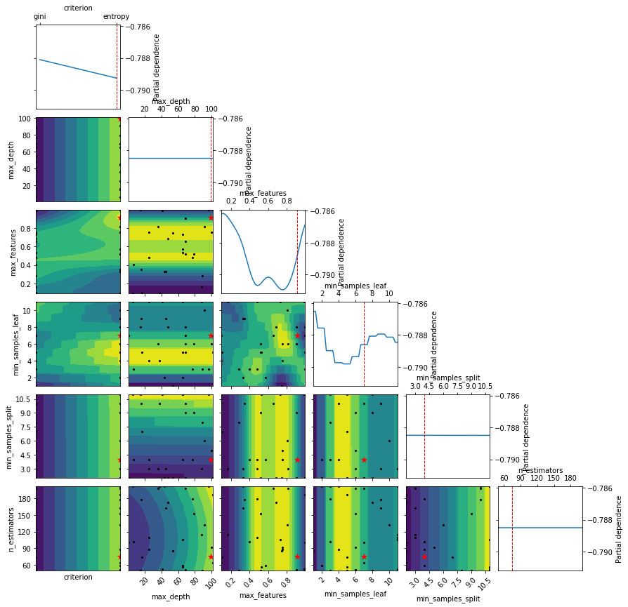
Show the partial dependency plot - an estimate of how features influence the objective function.

help(plot_objective)

[21]:

plot_objective(clf_bs.optimizer_results_[0],);

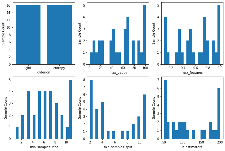
../_images/notebooks_B08_Hyperparameter_tuning_32_0.png

Show samples from the optimized space.

help(plot_histogram)

[22]:

fig, axes = plt.subplots(2,3,figsize=(12,8))
for i, ax in enumerate(axes.ravel()):
    plot_histogram(clf_bs.optimizer_results_[0], i, ax=ax);

../_images/notebooks_B08_Hyperparameter_tuning_34_0.png

Using `optuna`¶

[23]:

! python3 -m pip install --quiet optuna

[24]:

import optuna

[25]:

from sklearn.model_selection import cross_val_score

[26]:

class Objective(object):
    def __init__(self, X, y):
        self.X = X
        self.y = y

    def __call__(self, trial):
        X, y = self.X, self.y # load data once only

        criterion = trial.suggest_categorical('criterion', ['gini', 'entropy'])
        n_estimators = trial.suggest_int('n_estimators', 50, 201)
        max_features = trial.suggest_float('max_features', 1/p, 1)
        max_depth = trial.suggest_float('max_depth', 1, 128, log=True)
        min_samples_split = trial.suggest_int('min_samples_split', 2, 11, 1)
        min_samples_leaf = trial.suggest_int('min_samples_leaf', 1, 11, 1)

        clf = RandomForestClassifier(
            criterion = criterion,
            n_estimators = n_estimators,
            max_features = max_features,
            max_depth = max_depth,
            min_samples_split = min_samples_split,
            min_samples_leaf = min_samples_leaf,
        )

        score = cross_val_score(clf, X, y, n_jobs=-1,  cv=5).mean()
        return score

[27]:

optuna.logging.set_verbosity(0)

[28]:

%%time

objective1 = Objective(X_train, y_train)
study1 = optuna.create_study(direction='maximize')
study1.optimize(objective1, n_trials=N)

CPU times: user 500 ms, sys: 18.3 ms, total: 519 ms
Wall time: 7.68 s

[29]:

df_results1 = study1.trials_dataframe()

[30]:

df_results1.head(3)

[30]:

	number	value	datetime_start	datetime_complete	duration	params_criterion	params_max_depth	params_max_features	params_min_samples_leaf	params_min_samples_split	params_n_estimators	state
0	0	0.788998	2020-10-12 15:56:31.009453	2020-10-12 15:56:31.302377	0 days 00:00:00.292924	gini	68.068025	0.317078	7	8	175	COMPLETE
1	1	0.767590	2020-10-12 15:56:31.302410	2020-10-12 15:56:31.390874	0 days 00:00:00.088464	gini	2.318150	0.477432	7	3	63	COMPLETE
2	2	0.762488	2020-10-12 15:56:31.390903	2020-10-12 15:56:31.480004	0 days 00:00:00.089101	gini	1.036565	0.974324	4	8	62	COMPLETE

[31]:

from sklearn.model_selection import train_test_split

[32]:

class ObjectiveES(object):
    def __init__(self, X, y, max_iter=100):
        self.X_train, self.X_val, self.y_train, self.y_val = train_test_split(X, y)
        self.max_iter = max_iter

    def __call__(self, trial):
        # load ddta once only
        X_train, y_train, X_val, y_val = self.X_train, self.y_train, self.X_val, self.y_val

        criterion = trial.suggest_categorical('criterion', ['gini', 'entropy'])
        n_estimators = trial.suggest_int('n_estimators', 50, 201)
        max_features = trial.suggest_float('max_features', 1/p, 1)
        max_depth = trial.suggest_float('max_depth', 1, 128, log=True)
        min_samples_split = trial.suggest_int('min_samples_split', 2, 11, 1)
        min_samples_leaf = trial.suggest_int('min_samples_leaf', 1, 11, 1)

        clf = RandomForestClassifier(
            criterion = criterion,
            n_estimators = n_estimators,
            max_features = max_features,
            max_depth = max_depth,
            min_samples_split = min_samples_split,
            min_samples_leaf = min_samples_leaf,
        )

        for i in range(self.max_iter):
            clf.fit(X_train, y_train)
            score = clf.score(X_val, y_val)
            trial.report(score, i)
            if trial.should_prune():
                raise optuna.TrialPruned()
            return score

[33]:

%%time

objective2 = ObjectiveES(X_train, y_train)
study2 = optuna.create_study(direction='maximize')
study2.optimize(objective2, n_trials=N)

CPU times: user 6.63 s, sys: 24 ms, total: 6.65 s
Wall time: 6.66 s

[34]:

df_results2 = study2.trials_dataframe()
df_results2.head(3)

[34]:

	number	value	datetime_start	datetime_complete	duration	params_criterion	params_max_depth	params_max_features	params_min_samples_leaf	params_min_samples_split	params_n_estimators	state
0	0	0.813008	2020-10-12 15:56:38.736115	2020-10-12 15:56:38.915718	0 days 00:00:00.179603	entropy	10.027229	0.639109	11	9	87	COMPLETE
1	1	0.804878	2020-10-12 15:56:38.915750	2020-10-12 15:56:39.107483	0 days 00:00:00.191733	entropy	61.950795	0.343148	4	8	134	COMPLETE
2	2	0.841463	2020-10-12 15:56:39.107508	2020-10-12 15:56:39.359790	0 days 00:00:00.252282	entropy	60.831672	0.733779	2	7	152	COMPLETE

Visualizations¶

[35]:

from optuna.visualization import (plot_slice, plot_contour,
    plot_optimization_history,
    plot_param_importances,
    plot_parallel_coordinate
)

[36]:

plot_optimization_history(study2)

[37]:

plot_param_importances(study2)

[38]:

plot_contour(
    study2,
    ['min_samples_leaf', 'max_features', 'max_depth']
)

[39]:

plot_slice(study2, ['min_samples_leaf', 'max_features', 'max_depth'])

[40]:

plot_parallel_coordinate(study2, ['min_samples_leaf', 'max_features', 'max_depth'])

[41]:

clf_op1 = RandomForestClassifier(**study1.best_params)
clf_op1.fit(X_train, y_train)
clf_op2 = RandomForestClassifier(**study2.best_params)
clf_op2.fit(X_train, y_train);

[42]:

classifiers = [clf_gs, clf_rs1, clf_rs2, clf_bs, clf_op1, clf_op2]
names = ['Grid Search', 'Radnomized Search 1', 'Randomized Search 2',
         'Bayesian', 'Optuna', 'Optuna Pruned']

[43]:

for name, clf in zip(names, classifiers):
    print(f'{name:20s}: {clf.score(X_test, y_test): .3f}')

Grid Search         :  0.848
Radnomized Search 1 :  0.826
Randomized Search 2 :  0.841
Bayesian            :  0.829
Optuna              :  0.829
Optuna Pruned       :  0.823

Using `pycaret`¶

pycaret does not do anything that we have not done manually. However it presents a nice API that automates most of the boilerplate work in setting up a machine learning pipeline.

[44]:

! python3 -m pip install --quiet pycaret

[45]:

from pycaret.classification import (
    setup,
    compare_models,
    plot_model,
    create_model,
    tune_model,
    predict_model,
    stack_models,
    save_model,
    load_model,
)

[46]:

data = X_train.copy()
data['survived'] = y_train

[47]:

clfs = setup(
    data = data,
    target = 'survived',
    silent=True,
    session_id=1,
)

Setup Succesfully Completed!

	Description	Value
0	session_id	1
1	Target Type	Binary
2	Label Encoded	0: 0, 1: 1
3	Original Data	(981, 12)
4	Missing Values	False
5	Numeric Features	5
6	Categorical Features	6
7	Ordinal Features	False
8	High Cardinality Features	False
9	High Cardinality Method	None
10	Sampled Data	(981, 12)
11	Transformed Train Set	(686, 17)
12	Transformed Test Set	(295, 17)
13	Numeric Imputer	mean
14	Categorical Imputer	constant
15	Normalize	False
16	Normalize Method	None
17	Transformation	False
18	Transformation Method	None
19	PCA	False
20	PCA Method	None
21	PCA Components	None
22	Ignore Low Variance	False
23	Combine Rare Levels	False
24	Rare Level Threshold	None
25	Numeric Binning	False
26	Remove Outliers	False
27	Outliers Threshold	None
28	Remove Multicollinearity	False
29	Multicollinearity Threshold	None
30	Clustering	False
31	Clustering Iteration	None
32	Polynomial Features	False
33	Polynomial Degree	None
34	Trignometry Features	False
35	Polynomial Threshold	None
36	Group Features	False
37	Feature Selection	False
38	Features Selection Threshold	None
39	Feature Interaction	False
40	Feature Ratio	False
41	Interaction Threshold	None
42	Fix Imbalance	False
43	Fix Imbalance Method	SMOTE

[48]:

best_model = compare_models(sort = 'Accuracy')

	Model	Accuracy	AUC	Recall	Prec.	F1	Kappa	MCC	TT (Sec)
0	K Neighbors Classifier	0.8001	0.8192	0.6925	0.7477	0.7178	0.5637	0.5656	0.0031
1	CatBoost Classifier	0.7942	0.8443	0.6572	0.7560	0.7019	0.5463	0.5503	1.6133
2	Logistic Regression	0.7914	0.8271	0.6734	0.7426	0.7034	0.5437	0.5476	0.0155
3	Light Gradient Boosting Machine	0.7798	0.8298	0.6575	0.7300	0.6894	0.5198	0.5237	0.0375
4	Linear Discriminant Analysis	0.7797	0.8278	0.6772	0.7166	0.6936	0.5224	0.5251	0.0044
5	Gradient Boosting Classifier	0.7783	0.8246	0.6460	0.7317	0.6845	0.5146	0.5186	0.0926
6	Ridge Classifier	0.7768	0.0000	0.6694	0.7143	0.6881	0.5152	0.5183	0.0050
7	Extreme Gradient Boosting	0.7696	0.8223	0.6608	0.7016	0.6786	0.4995	0.5017	0.0808
8	Extra Trees Classifier	0.7564	0.7992	0.6534	0.6841	0.6662	0.4749	0.4772	0.1365
9	Random Forest Classifier	0.7506	0.8142	0.6215	0.6800	0.6456	0.4547	0.4586	0.0233
10	Ada Boost Classifier	0.7491	0.7955	0.6612	0.6659	0.6623	0.4629	0.4641	0.0783
11	SVM - Linear Kernel	0.7389	0.0000	0.6434	0.6666	0.6260	0.4332	0.4472	0.0050
12	Decision Tree Classifier	0.7361	0.7222	0.6657	0.6426	0.6503	0.4394	0.4431	0.0040
13	Naive Bayes	0.6704	0.8114	0.1402	0.8308	0.1891	0.1338	0.2157	0.0032
14	Quadratic Discriminant Analysis	0.6298	0.0000	0.0000	0.0000	0.0000	0.0000	0.0000	0.0028

[49]:

best_model

[49]:

KNeighborsClassifier(algorithm='auto', leaf_size=30, metric='minkowski',
                     metric_params=None, n_jobs=-1, n_neighbors=5, p=2,
                     weights='uniform')

[50]:

clf = create_model('gbc')

	Accuracy	AUC	Recall	Prec.	F1	Kappa	MCC
0	0.7681	0.8524	0.6538	0.7083	0.6800	0.4986	0.4996
1	0.8551	0.8945	0.6923	0.9000	0.7826	0.6767	0.6898
2	0.6812	0.7276	0.5385	0.5833	0.5600	0.3106	0.3112
3	0.7971	0.9222	0.6154	0.8000	0.6957	0.5473	0.5579
4	0.8551	0.8955	0.7600	0.8261	0.7917	0.6809	0.6822
5	0.7971	0.7905	0.6400	0.7619	0.6957	0.5452	0.5499
6	0.7647	0.7907	0.6000	0.7143	0.6522	0.4764	0.4806
7	0.6912	0.7660	0.5600	0.5833	0.5714	0.3302	0.3304
8	0.8088	0.7870	0.6800	0.7727	0.7234	0.5782	0.5810
9	0.7647	0.8200	0.7200	0.6667	0.6923	0.5023	0.5033
Mean	0.7783	0.8246	0.6460	0.7317	0.6845	0.5146	0.5186
SD	0.0556	0.0606	0.0662	0.0967	0.0723	0.1172	0.1196

[51]:

tuned_clf = tune_model(clf)

	Accuracy	AUC	Recall	Prec.	F1	Kappa	MCC
0	0.8116	0.8488	0.6154	0.8421	0.7111	0.5763	0.5919
1	0.8696	0.9244	0.6923	0.9474	0.8000	0.7067	0.7258
2	0.7101	0.7241	0.5000	0.6500	0.5652	0.3533	0.3602
3	0.8406	0.8927	0.6538	0.8947	0.7556	0.6415	0.6589
4	0.8696	0.8973	0.7200	0.9000	0.8000	0.7050	0.7147
5	0.8116	0.8250	0.6400	0.8000	0.7111	0.5739	0.5817
6	0.7500	0.7851	0.4800	0.7500	0.5854	0.4185	0.4399
7	0.7059	0.7651	0.5200	0.6190	0.5652	0.3455	0.3485
8	0.8088	0.8079	0.5600	0.8750	0.6829	0.5553	0.5837
9	0.7647	0.8400	0.6400	0.6957	0.6667	0.4853	0.4863
Mean	0.7942	0.8310	0.6022	0.7974	0.6843	0.5361	0.5492
SD	0.0566	0.0598	0.0785	0.1080	0.0847	0.1258	0.1291

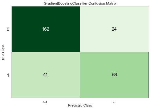
[52]:

plot_model(tuned_clf, 'confusion_matrix')

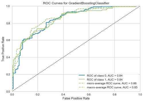
../_images/notebooks_B08_Hyperparameter_tuning_70_0.png

[53]:

plot_model(tuned_clf, 'auc')

../_images/notebooks_B08_Hyperparameter_tuning_72_0.png

[54]:

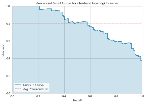
plot_model(tuned_clf, 'pr')

../_images/notebooks_B08_Hyperparameter_tuning_74_0.png

[55]:

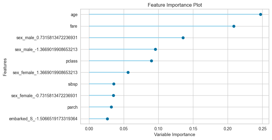
plot_model(tuned_clf, 'feature')

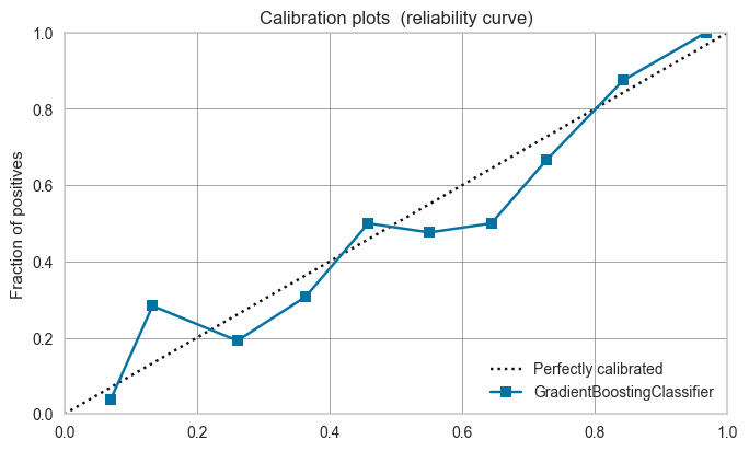
../_images/notebooks_B08_Hyperparameter_tuning_76_0.png

A calibration plot bins the test samples based on their predicted probabilities. If the predictions are good, the proportions should match the mean probability of the bin (i.e. be on the dotted line).

Models can be calibrated if the calibration plot shows a poor fit.

[56]:

plot_model(clf, plot='calibration')

../_images/notebooks_B08_Hyperparameter_tuning_79_0.png

[57]:

predict_model(clf);

	Model	Accuracy	AUC	Recall	Prec.	F1	Kappa	MCC
0	Gradient Boosting Classifier	0.7932	0.8614	0.6514	0.7553	0.6995	0.5432	0.5467

[58]:

predict_model(tuned_clf);

	Model	Accuracy	AUC	Recall	Prec.	F1	Kappa	MCC
0	Gradient Boosting Classifier	0.7797	0.8441	0.6239	0.7391	0.6766	0.5113	0.5156

We check a few other models.

[59]:

cb = create_model('catboost');

	Accuracy	AUC	Recall	Prec.	F1	Kappa	MCC
0	0.8261	0.8953	0.7308	0.7917	0.7600	0.6240	0.6252
1	0.8696	0.9329	0.7308	0.9048	0.8085	0.7113	0.7206
2	0.6812	0.7379	0.5000	0.5909	0.5417	0.2998	0.3023
3	0.8551	0.9258	0.7308	0.8636	0.7917	0.6817	0.6873
4	0.8841	0.9245	0.8000	0.8696	0.8333	0.7447	0.7462
5	0.7971	0.8168	0.6800	0.7391	0.7083	0.5532	0.5543
6	0.7500	0.8042	0.5600	0.7000	0.6222	0.4388	0.4449
7	0.7353	0.7930	0.5200	0.6842	0.5909	0.4006	0.4088
8	0.7941	0.7814	0.6400	0.7619	0.6957	0.5419	0.5466
9	0.7500	0.8307	0.6800	0.6538	0.6667	0.4668	0.4670
Mean	0.7942	0.8443	0.6572	0.7560	0.7019	0.5463	0.5503
SD	0.0622	0.0663	0.0954	0.0970	0.0926	0.1382	0.1383

[60]:

predict_model(cb);

	Model	Accuracy	AUC	Recall	Prec.	F1	Kappa	MCC
0	CatBoost Classifier	0.7831	0.8622	0.633	0.7419	0.6832	0.5198	0.5236

[61]:

tuned_cb = tune_model(cb)

	Accuracy	AUC	Recall	Prec.	F1	Kappa	MCC
0	0.8261	0.8819	0.7692	0.7692	0.7692	0.6297	0.6297
1	0.8841	0.9231	0.8077	0.8750	0.8400	0.7493	0.7508
2	0.7101	0.7366	0.5769	0.6250	0.6000	0.3733	0.3740
3	0.8406	0.9168	0.6923	0.8571	0.7660	0.6471	0.6556
4	0.8696	0.9218	0.7600	0.8636	0.8085	0.7102	0.7136
5	0.7681	0.8150	0.6000	0.7143	0.6522	0.4802	0.4843
6	0.7794	0.7716	0.5600	0.7778	0.6512	0.4960	0.5104
7	0.7647	0.8033	0.6400	0.6957	0.6667	0.4853	0.4863
8	0.8088	0.8233	0.6400	0.8000	0.7111	0.5709	0.5788
9	0.7353	0.8149	0.6800	0.6296	0.6538	0.4401	0.4409
Mean	0.7987	0.8408	0.6726	0.7607	0.7119	0.5582	0.5624
SD	0.0541	0.0629	0.0806	0.0877	0.0756	0.1167	0.1169

[62]:

predict_model(tuned_cb);

	Model	Accuracy	AUC	Recall	Prec.	F1	Kappa	MCC
0	CatBoost Classifier	0.7966	0.8636	0.6147	0.7882	0.6907	0.5426	0.552

[63]:

lr = create_model('lr');

	Accuracy	AUC	Recall	Prec.	F1	Kappa	MCC
0	0.7971	0.8453	0.6154	0.8000	0.6957	0.5473	0.5579
1	0.8116	0.8962	0.7308	0.7600	0.7451	0.5958	0.5961
2	0.6957	0.7039	0.5000	0.6190	0.5532	0.3264	0.3306
3	0.8841	0.9275	0.8077	0.8750	0.8400	0.7493	0.7508
4	0.8551	0.8755	0.8000	0.8000	0.8000	0.6864	0.6864
5	0.8261	0.8077	0.6800	0.8095	0.7391	0.6102	0.6154
6	0.7647	0.7995	0.6000	0.7143	0.6522	0.4764	0.4806
7	0.7206	0.7614	0.6800	0.6071	0.6415	0.4138	0.4156
8	0.7647	0.7749	0.5600	0.7368	0.6364	0.4672	0.4768
9	0.7941	0.8791	0.7600	0.7037	0.7308	0.5645	0.5656
Mean	0.7914	0.8271	0.6734	0.7426	0.7034	0.5437	0.5476
SD	0.0547	0.0660	0.0983	0.0805	0.0808	0.1203	0.1191

[64]:

predict_model(lr);

	Model	Accuracy	AUC	Recall	Prec.	F1	Kappa	MCC
0	Logistic Regression	0.7763	0.8417	0.6514	0.7172	0.6827	0.5105	0.5119

[65]:

tuned_lr = tune_model(lr)

	Accuracy	AUC	Recall	Prec.	F1	Kappa	MCC
0	0.7681	0.8488	0.7692	0.6667	0.7143	0.5208	0.5246
1	0.8116	0.8945	0.8462	0.7097	0.7719	0.6135	0.6204
2	0.6812	0.7039	0.6538	0.5667	0.6071	0.3411	0.3436
3	0.8841	0.9249	0.8846	0.8214	0.8519	0.7568	0.7582
4	0.8116	0.8764	0.8000	0.7143	0.7547	0.6026	0.6051
5	0.7826	0.8041	0.6800	0.7083	0.6939	0.5254	0.5257
6	0.7353	0.8060	0.7200	0.6207	0.6667	0.4491	0.4525
7	0.6912	0.7633	0.7200	0.5625	0.6316	0.3726	0.3810
8	0.7647	0.7758	0.6400	0.6957	0.6667	0.4853	0.4863
9	0.7794	0.8772	0.8400	0.6562	0.7368	0.5518	0.5643
Mean	0.7710	0.8275	0.7554	0.6722	0.7096	0.5219	0.5262
SD	0.0566	0.0651	0.0813	0.0731	0.0689	0.1152	0.1148

[66]:

predict_model(tuned_lr);

	Model	Accuracy	AUC	Recall	Prec.	F1	Kappa	MCC
0	Logistic Regression	0.7593	0.8422	0.7156	0.661	0.6872	0.4921	0.4932

[67]:

top = compare_models(n_select = 5)

	Model	Accuracy	AUC	Recall	Prec.	F1	Kappa	MCC	TT (Sec)
0	K Neighbors Classifier	0.8001	0.8192	0.6925	0.7477	0.7178	0.5637	0.5656	0.0030
1	CatBoost Classifier	0.7942	0.8443	0.6572	0.7560	0.7019	0.5463	0.5503	1.6453
2	Logistic Regression	0.7914	0.8271	0.6734	0.7426	0.7034	0.5437	0.5476	0.0146
3	Light Gradient Boosting Machine	0.7798	0.8298	0.6575	0.7300	0.6894	0.5198	0.5237	0.0358
4	Linear Discriminant Analysis	0.7797	0.8278	0.6772	0.7166	0.6936	0.5224	0.5251	0.0045
5	Gradient Boosting Classifier	0.7783	0.8246	0.6460	0.7317	0.6845	0.5146	0.5186	0.0944
6	Ridge Classifier	0.7768	0.0000	0.6694	0.7143	0.6881	0.5152	0.5183	0.0046
7	Extreme Gradient Boosting	0.7696	0.8223	0.6608	0.7016	0.6786	0.4995	0.5017	0.0822
8	Extra Trees Classifier	0.7564	0.7992	0.6534	0.6841	0.6662	0.4749	0.4772	0.1305
9	Random Forest Classifier	0.7506	0.8142	0.6215	0.6800	0.6456	0.4547	0.4586	0.0232
10	Ada Boost Classifier	0.7491	0.7955	0.6612	0.6659	0.6623	0.4629	0.4641	0.0779
11	SVM - Linear Kernel	0.7389	0.0000	0.6434	0.6666	0.6260	0.4332	0.4472	0.0050
12	Decision Tree Classifier	0.7361	0.7222	0.6657	0.6426	0.6503	0.4394	0.4431	0.0040
13	Naive Bayes	0.6704	0.8114	0.1402	0.8308	0.1891	0.1338	0.2157	0.0034
14	Quadratic Discriminant Analysis	0.6298	0.0000	0.0000	0.0000	0.0000	0.0000	0.0000	0.0033

[68]:

stack_clf = stack_models(top)

	Accuracy	AUC	Recall	Prec.	F1	Kappa	MCC
0	0.8406	0.8801	0.7308	0.8261	0.7755	0.6526	0.6556
1	0.8696	0.9222	0.7308	0.9048	0.8085	0.7113	0.7206
2	0.7101	0.7030	0.5769	0.6250	0.6000	0.3733	0.3740
3	0.8696	0.9222	0.7692	0.8696	0.8163	0.7158	0.7190
4	0.8841	0.9009	0.8000	0.8696	0.8333	0.7447	0.7462
5	0.7826	0.8186	0.6400	0.7273	0.6809	0.5170	0.5195
6	0.7500	0.8312	0.6000	0.6818	0.6383	0.4485	0.4506
7	0.7647	0.7763	0.6000	0.7143	0.6522	0.4764	0.4806
8	0.8088	0.7842	0.6400	0.8000	0.7111	0.5709	0.5788
9	0.7794	0.8586	0.7200	0.6923	0.7059	0.5295	0.5298
Mean	0.8059	0.8397	0.6808	0.7711	0.7222	0.5740	0.5775
SD	0.0554	0.0676	0.0747	0.0904	0.0778	0.1204	0.1215

[69]:

predict_model(stack_clf);

	Model	Accuracy	AUC	Recall	Prec.	F1	Kappa	MCC
0	Stacking Classifier	0.7898	0.8634	0.6514	0.7474	0.6961	0.5366	0.5396

[70]:

import pendulum

[71]:

today = pendulum.today()

[72]:

save_model(tuned_cb, f'Titanic Tuned CatBoost {today}')

Transformation Pipeline and Model Succesfully Saved

[73]:

!ls T*

Titanic Tuned CatBoost 2020-10-12T00:00:00-04:00.pkl

[74]:

clf = load_model(f'Titanic Tuned CatBoost {today}')

Transformation Pipeline and Model Successfully Loaded

[75]:

predict_model(tuned_cb);

	Model	Accuracy	AUC	Recall	Prec.	F1	Kappa	MCC
0	CatBoost Classifier	0.7966	0.8636	0.6147	0.7882	0.6907	0.5426	0.552

[76]:

predict_model(clf);

	Model	Accuracy	AUC	Recall	Prec.	F1	Kappa	MCC
0	CatBoost Classifier	0.7966	0.8636	0.6147	0.7882	0.6907	0.5426	0.552

[ ]: