[1]:
%matplotlib inline
import matplotlib as mpl
import matplotlib.pyplot as plt
import numpy as np
import pandas as pd
[2]:
from sklearn.cluster import KMeans
from sklearn.metrics import adjusted_mutual_info_score
[3]:
from sklearn.datasets import make_blobs
[4]:
plt.style.use('dark_background')
Clustering
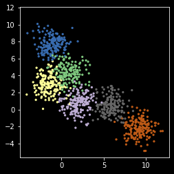
Toy example to illustrate concepts
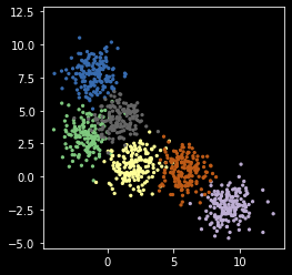
[5]:
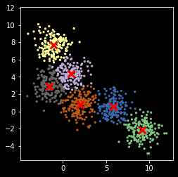
npts = 1000
nc = 6
X, y = make_blobs(n_samples=npts, centers=nc, random_state=0)
[6]:
plt.scatter(X[:, 0], X[:, 1], s=5, c=y,
            cmap=plt.cm.get_cmap('Accent', nc))
plt.axis('square')
pass
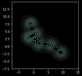
Sometimes the structure is clearer with contours
[7]:
import seaborn as sns
[8]:
sns.kdeplot(X[:, 0], X[:, 1])
plt.axis('square');
How to cluster
Choose a clustering algorithm
Choose the number of clusters
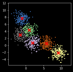
Using a library function
Normally, we would use a library function. The examples below are meant to illustrate how the k-means algorithm works.
[9]:
kmeans = KMeans(nc)
[10]:
z = kmeans.fit_predict(X)
centers = kmeans.cluster_centers_
[11]:
plt.scatter(X[:, 0], X[:, 1], s=5, c=z,
            cmap=plt.cm.get_cmap('Accent', nc))
plt.scatter(centers[:, 0], centers[:, 1], marker='x',
            linewidth=3, s=100, c='red')
plt.axis('square')
pass
Coding from the ground up
There are many different clustering methods, but K-means is fast, scales well, and can be interpreted as a probabilistic model. We will write 3 versions of the K-means algorithm to illustrate the main concepts. The algorithm is very simple:
Start with \(k\) centers with labels \(0, 1, \ldots, k-1\)
Find the distance of each data point to each center
Assign the data points nearest to a center to its label
Use the mean of the points assigned to a center as the new center
Repeat for a fixed number of iterations or until the centers stop changing
Note: If you want a probabilistic interpretation, just treat the final solution as a mixture of (multivariate) normal distributions. K-means is often used to initialize the fitting of full statistical mixture models, which are computationally more demanding and hence slower.
Distance between sets of vectors
[12]:
from scipy.spatial.distance import cdist
[13]:
pts = np.arange(6).reshape(-1,2)
pts
[13]:
array([[0, 1],
       [2, 3],
       [4, 5]])
[14]:
mus = np.arange(4).reshape(-1, 2)
mus
[14]:
array([[0, 1],
       [2, 3]])
[15]:
cdist(pts, mus)
[15]:
array([[0.        , 2.82842712],
       [2.82842712, 0.        ],
       [5.65685425, 2.82842712]])
Version 1
[16]:
def my_kemans_1(X, k, iters=10):
    """K-means with fixed number of iterations."""

    r, c = X.shape
    centers = X[np.random.choice(r, k, replace=False)]
    for i in range(iters):
        m = cdist(X, centers)
        z = np.argmin(m, axis=1)
        centers = np.array([np.mean(X[z==i], axis=0) for i in range(k)])
    return (z, centers)
[17]:
np.random.seed(2018)
z, centers = my_kemans_1(X, nc)
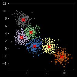
Note that K-means can get stuck in local optimum
[18]:
plt.scatter(X[:, 0], X[:, 1], s=5, c=z,
            cmap=plt.cm.get_cmap('Accent', nc))
plt.scatter(centers[:, 0], centers[:, 1], marker='x',
            linewidth=3, s=100, c='red')
plt.axis('square')
pass
Version 2
[19]:
def my_kemans_2(X, k, tol= 1e-6):
    """K-means with tolerance."""

    r, c = X.shape
    centers = X[np.random.choice(r, k, replace=False)]
    delta = np.infty
    while delta > tol:
        m = cdist(X, centers)
        z = np.argmin(m, axis=1)
        new_centers = np.array([np.mean(X[z==i], axis=0) for i in range(k)])
        delta = np.sum((new_centers - centers)**2)
        centers = new_centers
    return (z, centers)
[20]:
np.random.seed(2018)
z, centers = my_kemans_2(X, nc)
Still stuck in local optimum
[21]:
plt.scatter(X[:, 0], X[:, 1], s=5, c=z,
            cmap=plt.cm.get_cmap('Accent', nc))
plt.scatter(centers[:, 0], centers[:, 1], marker='x',
            linewidth=3, s=100, c='red')
plt.axis('square')
pass

Version 3
Use of a score to evaluate the goodness of fit. In this case, the simplest score is just the sum of distances from each point to its nearest center.
[22]:
def my_kemans_3(X, k, tol=1e-6, n_starts=10):
    """K-means with tolerance and random restarts."""

    r, c = X.shape
    best_score = np.infty

    for i in range(n_starts):
        centers = X[np.random.choice(r, k, replace=False)]
        delta = np.infty
        while delta > tol:
            m = cdist(X, centers)
            z = np.argmin(m, axis=1)
            new_centers = np.array([np.mean(X[z==i], axis=0) for i in range(k)])
            delta = np.sum((new_centers - centers)**2)
            centers = new_centers
        score = m[z].sum()
        if score < best_score:
            best_score = score
            best_z = z
            best_centers = centers
    return (best_z, best_centers)
[23]:
np.random.seed(2018)
z, centers = my_kemans_3(X, nc)
[24]:
plt.scatter(X[:, 0], X[:, 1], s=5, c=z,
            cmap=plt.cm.get_cmap('Accent', nc))
plt.scatter(centers[:, 0], centers[:, 1], marker='x',
            linewidth=3, s=100, c='red')
plt.axis('square')
pass
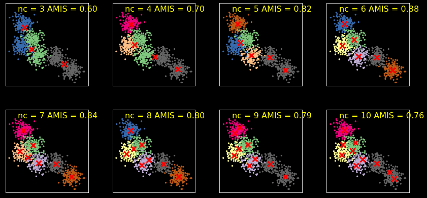
Model selection
We use AMIS for model selection. You can also use likelihood-based methods by interpreting the solution as a mixture of normals but we don’t cover those approaches here. There are also other ad-hoc methods - see sckikt-lean docs if you are interested.
The mutual information is defined as
It measures how much knowing \(X\) reduces the uncertainty about \(Y\) (and vice versa).
If \(X\) is independent of \(Y\), then \(I(X; Y) = 0\)
If \(X\) is a deterministic function of \(Y\), then \(I(X; Y) = 1\)
It is equivalent to the Kullback-Leibler divergence
We use AMIS (Adjusted MIS) here, which adjusts for the number of clusters used in the clustering method.
From the documentation
AMI(U, V) = [MI(U, V) - E(MI(U, V))] / [max(H(U), H(V)) - E(MI(U, V))]
[25]:
ncols = 4
nrows = 2
plt.figure(figsize=(ncols*3, nrows*3))
for i, nc in enumerate(range(3, 11)):
    kmeans = KMeans(nc, n_init=10)
    clusters = kmeans.fit_predict(X)
    centers = kmeans.cluster_centers_
    amis = adjusted_mutual_info_score(y, clusters)
    plt.subplot(nrows, ncols, i+1)
    plt.scatter(X[:, 0], X[:, 1], s=5, c=y,
                cmap=plt.cm.get_cmap('Accent', nc))
    plt.scatter(centers[:, 0], centers[:, 1], marker='x',
                linewidth=3, s=100, c='red')
    plt.text(0.15, 0.9, 'nc = %d AMIS = %.2f' % (nc, amis),
             fontsize=16, color='yellow',
             transform=plt.gca().transAxes)
    plt.xticks([])
    plt.yticks([])
    plt.axis('square')
plt.tight_layout()
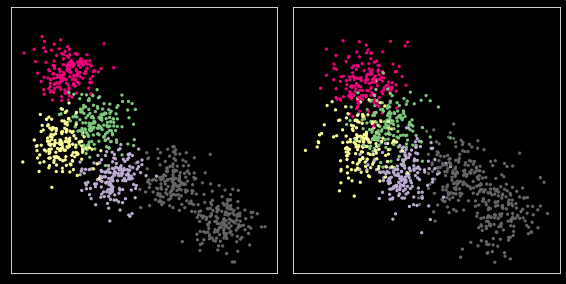
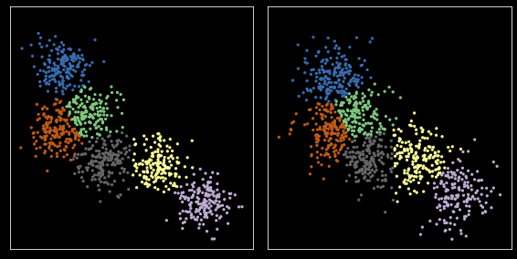
Comparing across samples
[26]:
X1 = X + np.random.normal(0, 1, X.shape)
[27]:
plt.figure(figsize=(8, 4))
for i, xs in enumerate([X, X1]):
    plt.subplot(1,2,i+1)
    plt.scatter(xs[:, 0], xs[:, 1], s=5, c=y,
                cmap=plt.cm.get_cmap('Accent', nc))
    plt.xticks([])
    plt.yticks([])
    plt.axis('square')
plt.tight_layout()
pass
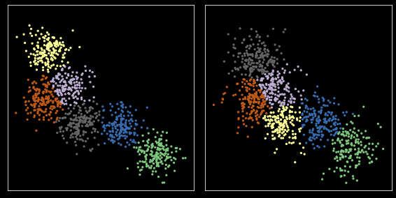
[28]:
nc = 6
kmeans = KMeans(nc, n_init=10)
kmeans.fit(X)
z1 = kmeans.predict(X)
z2 = kmeans.predict(X1)
zs = [z1, z2]
[29]:
plt.figure(figsize=(8, 4))
for i, xs in enumerate([X, X1]):
    plt.subplot(1,2,i+1)
    plt.scatter(xs[:, 0], xs[:, 1], s=5, c=zs[i],
                cmap=plt.cm.get_cmap('Accent', nc))
    plt.xticks([])
    plt.yticks([])
    plt.axis('square')
plt.tight_layout()
pass
[30]:
Y = np.r_[X, X1]
kmeans = KMeans(nc, n_init=10)
kmeans.fit(Y)
zs = np.split(kmeans.predict(Y), 2)
[31]:
plt.figure(figsize=(8, 4))
for i, xs in enumerate([X, X1]):
    plt.subplot(1,2,i+1)
    plt.scatter(xs[:, 0], xs[:, 1], s=5, c=zs[i],
                cmap=plt.cm.get_cmap('Accent', nc))
    plt.xticks([])
    plt.yticks([])
    plt.axis('square')
plt.tight_layout()
pass
[32]:
from scipy.optimize import linear_sum_assignment
[33]:
np.random.seed(2018)
kmeans = KMeans(nc, n_init=10)
c1 = kmeans.fit(X).cluster_centers_
z1 = kmeans.predict(X)
c2 = kmeans.fit(X1).cluster_centers_
z2 = kmeans.predict(X1)
zs = [z1, z2]
cs = [c1, c2]
[34]:
plt.figure(figsize=(8, 4))
for i, xs in enumerate([X, X1]):
    plt.subplot(1,2,i+1)
    z = zs[i]
    c = cs[i]

    plt.scatter(xs[:, 0], xs[:, 1], s=5, c=z,
                cmap=plt.cm.get_cmap('Accent', nc))
    plt.xticks([])
    plt.yticks([])
    plt.axis('square')
plt.tight_layout()
pass
Define cost function
We use a simple cost as just the distance between centers. More complex dissimilarity measures could be used.
[35]:
cost = cdist(c1, c2)
Run the Hungarian (Muunkres) algorithm for bipartitie matching
[36]:
row_ind, col_ind = linear_sum_assignment(cost)
[37]:
row_ind, col_ind
[37]:
(array([0, 1, 2, 3, 4, 5]), array([0, 1, 5, 3, 4, 2]))
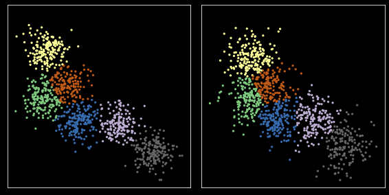
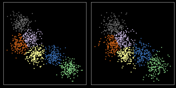
Swap cluster indexes to align data sets
[38]:
z1_aligned = col_ind[z1]
zs = [z1_aligned, z2]
[39]:
plt.figure(figsize=(8, 4))
for i, xs in enumerate([X, X1]):
    plt.subplot(1,2,i+1)
    plt.scatter(xs[:, 0], xs[:, 1], s=5, c=zs[i],
                cmap=plt.cm.get_cmap('Accent', nc))
    plt.xticks([])
    plt.yticks([])
    plt.axis('square')
plt.tight_layout()
pass
Probabilistic alternatives to k-means
There are several advantages to fitting a probabilistic model:
There is a probabilistic interpretation
It is generative
You have a log likelihood to work with - e.g. evaluate model fit with AIC and BIC
[40]:
from sklearn.mixture import GaussianMixture
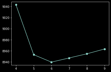
Model selection
We can use so-called information criteria that approximate the leave-one-out error. Two commonly used are
AIC - Akaike Information Criteria
BIC - Bayesian Information Criteria
Basically, they add a penalty term to the negative log likelihood to penalize for model complexity. BIC is generally more conservative than AIC (i.e. BIC prefers less complex models).
[41]:
aics = []
bics = []
for i in range(4, 10):
    gmm = GaussianMixture(n_components=i)
    gmm.fit(X)
    aics.append(gmm.aic(X))
    bics.append(gmm.bic(X))
[42]:
min(list(zip(range(4,10), aics)), key = lambda x: x[1])
[42]:
(6, 8939.46780097899)
[43]:
plt.plot(range(4, 10), aics, '-o');
[44]:
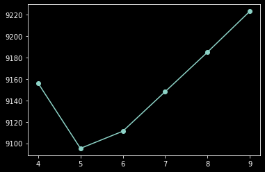
min(list(zip(range(4,10), bics)), key = lambda x: x[1])
[44]:
(5, 9095.225715313982)
[45]:
plt.plot(range(4, 10), bics, '-o');
Generative model
You can draw synthetic samples from the fitted distribution.
[46]:
gmm = GaussianMixture(n_components=nc)
gmm.fit(X)
xs, zs = gmm.sample(1000)
[47]:
plt.scatter(xs[:, 0], xs[:, 1], s=5, c=zs,
            cmap=plt.cm.get_cmap('Accent', nc))
plt.axis('square')
pass
[ ]: