Deep Learning Models
This is not a deep learning course, but by request, I will introduce simple examples to get started in deep learning and highlight some aspects that I find interesting. In particular, strategies for optimization and specialized architectures are not covered.
[1]:
%matplotlib inline
[2]:
import warnings
warnings.simplefilter('ignore', RuntimeWarning)
[3]:
import matplotlib.pyplot as plt
import pandas as pd
import numpy as np
import seaborn as sns
[4]:
import tensorflow as tf
import tensorflow.keras as keras
[5]:
from tensorflow.keras.layers.experimental import preprocessing
[6]:
from tensorflow.keras.utils import plot_model
[7]:
import tensorflow_datasets as tfds
Building models
Prepare data
[8]:
(ds_train, ds_val), info = tfds.load(
    'iris',
    split=[
       'train[:70%]',
       'train[70%:]'
    ],
    batch_size=8,
    with_info=True,
    as_supervised=True,
)
[9]:
for row, label in ds_train.take(1):
    print(row.numpy())
    print(label.numpy())
[[5.1 3.4 1.5 0.2]
 [7.7 3.  6.1 2.3]
 [5.7 2.8 4.5 1.3]
 [6.8 3.2 5.9 2.3]
 [5.2 3.4 1.4 0.2]
 [5.6 2.9 3.6 1.3]
 [5.5 2.6 4.4 1.2]
 [5.5 2.4 3.7 1. ]]
[0 2 1 2 0 1 1 1]
[10]:
shape = info.features.shape['features']
Pre-process data
If you need to pre-process your data, see https://keras.io/api/preprocessing/. We will not do any pre-processing for simplicity.
Sequential API
If the entire pipeline is a single chain of layers, the Sequential API is the simplest to use.
[11]:
from tensorflow.keras.models import Sequential, Model
from tensorflow.keras.layers import Dense, Input, concatenate
Set random seed for reproducibility
[12]:
np.random.seed(0)
tf.random.set_seed(0)
[13]:
model = Sequential()
model.add(Dense(8, input_shape=shape))
model.add(Dense(4, activation='relu'))
model.add(Dense(3, activation='softmax'))
Alternative model specification
model = Sequential(
    Dense(8, input_shape=(4,)),
    Dense(4, activation='relu'),
    Dense(3, activation='softmax')
)
[14]:
model.compile(
    optimizer='adam',
    loss='sparse_categorical_crossentropy',
    metrics=['accuracy']
)
[15]:
model.summary()
Model: "sequential"
_________________________________________________________________
Layer (type)                 Output Shape              Param #
=================================================================
dense (Dense)                (None, 8)                 40
_________________________________________________________________
dense_1 (Dense)              (None, 4)                 36
_________________________________________________________________
dense_2 (Dense)              (None, 3)                 15
=================================================================
Total params: 91
Trainable params: 91
Non-trainable params: 0
_________________________________________________________________
[16]:
hist = model.fit(
    ds_train,
    validation_data=ds_val,
    epochs=50,
    verbose=0)
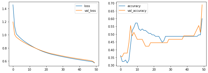
[17]:
fig, axes = plt.subplots(1,2,figsize=(12, 4))
for ax, measure in zip(axes, ['loss', 'accuracy']):
    ax.plot(hist.history[measure], label=measure)
    ax.plot(hist.history['val_' + measure], label='val_' + measure)
    ax.legend()
pass
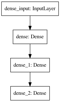
[18]:
plot_model(model)
[18]:
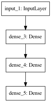
Functional API
The functional API provides flexibility, allowing you to build models with multiple inputs, multiple outputs, or branch and merge architectures.
Set random seed for reproducibility
[19]:
np.random.seed(0)
tf.random.set_seed(0)
[20]:
input = Input(shape=(4,))
x = Dense(8)(input)
x = Dense(4, activation='relu')(x)
output = Dense(3, activation='softmax')(x)
model = Model(inputs=[input], outputs=[output])
[21]:
model.compile(
    optimizer='adam',
    loss='sparse_categorical_crossentropy',
    metrics=['accuracy']
)
[22]:
model.summary()
Model: "functional_1"
_________________________________________________________________
Layer (type)                 Output Shape              Param #
=================================================================
input_1 (InputLayer)         [(None, 4)]               0
_________________________________________________________________
dense_3 (Dense)              (None, 8)                 40
_________________________________________________________________
dense_4 (Dense)              (None, 4)                 36
_________________________________________________________________
dense_5 (Dense)              (None, 3)                 15
=================================================================
Total params: 91
Trainable params: 91
Non-trainable params: 0
_________________________________________________________________
[23]:
hist = model.fit(
    ds_train,
    validation_data=ds_val,
    epochs=50,
    verbose=0)
[24]:
fig, axes = plt.subplots(1,2,figsize=(12, 4))
for ax, measure in zip(axes, ['loss', 'accuracy']):
    ax.plot(hist.history[measure], label=measure)
    ax.plot(hist.history['val_' + measure], label='val_' + measure)
    ax.legend()
pass

[25]:
plot_model(model)
[25]:
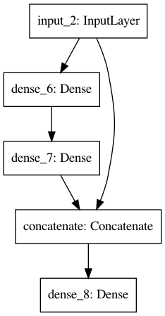
Flexibility of functional API
You can easily implement multiple inputs, multiple outputs or skip connections. Note that if you have multiple outputs, you probably also want multiple loss functions given as a list in the compile step (unless the same loss function is applicable to both outputs).
[26]:
input = Input(shape=(4,))
x1 = Dense(8)(input)
x2 = Dense(4, activation='relu')(x1)
x3 = concatenate([input, x2])
output = Dense(3, activation='softmax')(x3)
model = Model(inputs=[input], outputs=[output])
[27]:
plot_model(model)
[27]:
Built-in models and transfer learning
Keras comes with many built-in model architectures that serve as great starting points. Sometimes they even come pre-trained on massive data sets and can be used out-of-the-box, or improved with some transfer learning.
[28]:
ds, info = tfds.load(name='fashion_mnist',
                     as_supervised=True,
                     batch_size=32,
                     with_info=True)
[29]:
from tensorflow.keras.applications.inception_v3 import InceptionV3
from tensorflow.keras.layers import Input, Dense, GlobalAveragePooling2D
from tensorflow.keras.models import Model
[30]:
size = [75, 75]
X_train = (ds['train'].
           map(lambda image, label:
               (tf.image.resize(tf.image.grayscale_to_rgb(image), size), label)))
X_test = (ds['test'].
          map(lambda image, label:
              (tf.image.resize(tf.image.grayscale_to_rgb(image), size), label)))
[31]:
shape = [item[0].shape for item in X_train.take(1)][0]
shape
[31]:
TensorShape([32, 75, 75, 3])
[32]:
base_model = InceptionV3(
    input_shape=shape[1:],
    weights='imagenet',
    include_top=False,
    classes=10
)
I will plot the model architecture to show why this is deep learning.
[33]:
plot_model(base_model)
[33]:
[34]:
for layer in base_model.layers:
    layer.trainable = False
[35]:
x = base_model.output
x = GlobalAveragePooling2D()(x)
x = Dense(1024, activation='relu')(x)
output = Dense(10, activation='softmax')(x)
model = Model(inputs=base_model.input, outputs=output)
[36]:
model.compile(
    optimizer='adam',
    loss='sparse_categorical_crossentropy',
    metrics=['accuracy']
)
[37]:
model.fit(X_train, epochs=5)
Epoch 1/5
1875/1875 [==============================] - 160s 85ms/step - loss: 3.3702 - accuracy: 0.6858
Epoch 2/5
1875/1875 [==============================] - 164s 87ms/step - loss: 0.7235 - accuracy: 0.7334
Epoch 3/5
1875/1875 [==============================] - 164s 87ms/step - loss: 0.6897 - accuracy: 0.7462
Epoch 4/5
1875/1875 [==============================] - 163s 87ms/step - loss: 0.6730 - accuracy: 0.7539
Epoch 5/5
1875/1875 [==============================] - 161s 86ms/step - loss: 0.6513 - accuracy: 0.7598
[37]:
<tensorflow.python.keras.callbacks.History at 0x153c41550>
[38]:
test_loss, test_acc = model.evaluate(X_test)
test_acc
313/313 [==============================] - 25s 81ms/step - loss: 0.6809 - accuracy: 0.7578
[38]:
0.7577999830245972
Custom methods
It is not hard to develop custom methods for keras, which you might need if you are developing your own methods or want to adapt an existing method from the literature. A few examples are shown to give you an idea of how easy it generally is to write your own custom methods.
Custom learning rate
[39]:
def custom_lr(epoch):
    if epoch < 3:
        return 0.001
    else:
        return 0.0001
[40]:
schedule = keras.callbacks.LearningRateScheduler(custom_lr)
[41]:
model.fit(X_train, epochs=5, callbacks=[schedule])
Epoch 1/5
1875/1875 [==============================] - 167s 89ms/step - loss: 0.6423 - accuracy: 0.7632
Epoch 2/5
1875/1875 [==============================] - 165s 88ms/step - loss: 0.6312 - accuracy: 0.7697
Epoch 3/5
1875/1875 [==============================] - 172s 91ms/step - loss: 0.6213 - accuracy: 0.7713
Epoch 4/5
1875/1875 [==============================] - 173s 92ms/step - loss: 0.5313 - accuracy: 0.8014
Epoch 5/5
1875/1875 [==============================] - 171s 91ms/step - loss: 0.5198 - accuracy: 0.8047
[41]:
<tensorflow.python.keras.callbacks.History at 0x153e13f10>
Custom loss functions
It is very easy to create a custom loss.
Note: If you need to also save and load a model with a custom loss, you need to wrap it up in a class. See official documentation for details (mostly boilerplate code).
[42]:
def custom_loss(y_true, y_pred):
    error = y_true - y_pred
    return tf.pow(error, 1.5)
[43]:
model.compile(
    optimizer='adam',
    loss=custom_loss,
    metrics=['accuracy']
)
Custom metrics
This is very similar to a loss function. The main difference is that metrics should be human interpretable.
[44]:
def custom_metric(y_true, y_pred):
    error = y_true - y_pred
    return tf.abs(eror) - 0.5
[45]:
model.compile(
    optimizer='adam',
    loss=custom_loss,
    metrics=['accuracy', custom_metric]
)
Custom activation function
[46]:
def custom_activation(z):
    return tf.math.log(1.0 + tf.exp(z))
[47]:
layer = Dense(1, activation=custom_activation)
Hyperparameter optimization
[48]:
import optuna
[49]:
from tensorflow.keras.layers import Conv2D, MaxPooling2D, Dropout, Flatten
[50]:
(X_train, y_train), (X_test, y_test) = tf.keras.datasets.mnist.load_data()
X_train, X_test = X_train / 255.0, X_test / 255.0
X_train = X_train.astype('float32')
X_test = X_test.astype('float32')
X_train = X_train.reshape(X_train.shape[0], 28, 28, 1)
X_test = X_test.reshape(X_test.shape[0], 28, 28, 1)
[51]:
class Objective(object):
    def __init__(self, X, y,
                 max_epochs,
                 input_shape,
                 num_classes):
        self.X = X
        self.y = y
        self.max_epochs = max_epochs
        self.input_shape = input_shape
        self.num_classes = num_classes

    def __call__(self, trial):
        dropout=trial.suggest_discrete_uniform('dropout', 0.05, 0.5, 0.05)
        batch_size = trial.suggest_categorical('batch_size', [32, 64, 96, 128])

        params = dict(
            dropout = dropout,
            batch_size = batch_size
        )

        model = Sequential()
        model.add(Conv2D(32, kernel_size=(3, 3),
                         activation='relu',
                         input_shape=self.input_shape))
        model.add(Conv2D(64, (3, 3), activation='relu'))
        model.add(MaxPooling2D(pool_size=(2, 2)))
        model.add(Dropout(params['dropout']))
        model.add(Flatten())
        model.add(Dense(128, activation='relu'))
        model.add(Dropout(params['dropout']))
        model.add(Dense(self.num_classes, activation='softmax'))

        model.compile(optimizer='adam',
                      loss='sparse_categorical_crossentropy',
                      metrics=['accuracy'])

        # fit the model
        hist = model.fit(x=self.X, y=self.y,
                          batch_size=params['batch_size'],
                          validation_split=0.25,
                          epochs=self.max_epochs)

        loss = np.min(hist.history['val_loss'])

        return loss
[52]:
optuna.logging.set_verbosity(0)
[53]:
N = 5
max_epochs = 3
input_shape = (28,28,1)
num_classes = 10
[54]:
%%time

objective1 = Objective(X_train, y_train, max_epochs, input_shape, num_classes)
study1 = optuna.create_study(direction='minimize')
study1.optimize(objective1, n_trials=N)
Epoch 1/3
469/469 [==============================] - 31s 67ms/step - loss: 0.2097 - accuracy: 0.9364 - val_loss: 0.0660 - val_accuracy: 0.9805
Epoch 2/3
469/469 [==============================] - 32s 67ms/step - loss: 0.0718 - accuracy: 0.9777 - val_loss: 0.0529 - val_accuracy: 0.9845
Epoch 3/3
469/469 [==============================] - 32s 67ms/step - loss: 0.0487 - accuracy: 0.9845 - val_loss: 0.0474 - val_accuracy: 0.9870
Epoch 1/3
469/469 [==============================] - 32s 67ms/step - loss: 0.1825 - accuracy: 0.9440 - val_loss: 0.0620 - val_accuracy: 0.9815
Epoch 2/3
469/469 [==============================] - 32s 68ms/step - loss: 0.0526 - accuracy: 0.9839 - val_loss: 0.0486 - val_accuracy: 0.9847
Epoch 3/3
469/469 [==============================] - 32s 69ms/step - loss: 0.0324 - accuracy: 0.9897 - val_loss: 0.0480 - val_accuracy: 0.9859
Epoch 1/3
469/469 [==============================] - 33s 70ms/step - loss: 0.1970 - accuracy: 0.9402 - val_loss: 0.0655 - val_accuracy: 0.9803
Epoch 2/3
469/469 [==============================] - 33s 70ms/step - loss: 0.0581 - accuracy: 0.9825 - val_loss: 0.0466 - val_accuracy: 0.9855
Epoch 3/3
469/469 [==============================] - 33s 70ms/step - loss: 0.0392 - accuracy: 0.9879 - val_loss: 0.0505 - val_accuracy: 0.9854
Epoch 1/3
469/469 [==============================] - 33s 70ms/step - loss: 0.2069 - accuracy: 0.9377 - val_loss: 0.0619 - val_accuracy: 0.9823
Epoch 2/3
469/469 [==============================] - 33s 70ms/step - loss: 0.0671 - accuracy: 0.9799 - val_loss: 0.0519 - val_accuracy: 0.9853
Epoch 3/3
469/469 [==============================] - 33s 71ms/step - loss: 0.0485 - accuracy: 0.9853 - val_loss: 0.0481 - val_accuracy: 0.9854
Epoch 1/3
704/704 [==============================] - 38s 54ms/step - loss: 0.1939 - accuracy: 0.9401 - val_loss: 0.0605 - val_accuracy: 0.9819
Epoch 2/3
704/704 [==============================] - 36s 51ms/step - loss: 0.0713 - accuracy: 0.9779 - val_loss: 0.0465 - val_accuracy: 0.9869
Epoch 3/3
704/704 [==============================] - 36s 52ms/step - loss: 0.0513 - accuracy: 0.9840 - val_loss: 0.0484 - val_accuracy: 0.9858
CPU times: user 54min 14s, sys: 5min 26s, total: 59min 40s
Wall time: 8min 20s
[55]:
df = study1.trials_dataframe()
[56]:
df.head()
[56]:
| number | value | datetime_start | datetime_complete | duration | params_batch_size | params_dropout | state | |
|---|---|---|---|---|---|---|---|---|
| 0 | 0 | 0.047400 | 2020-10-21 09:16:39.312276 | 2020-10-21 09:18:14.498391 | 0 days 00:01:35.186115 | 96 | 0.30 | COMPLETE |
| 1 | 1 | 0.047991 | 2020-10-21 09:18:14.498431 | 2020-10-21 09:19:50.615475 | 0 days 00:01:36.117044 | 96 | 0.15 | COMPLETE |
| 2 | 2 | 0.046602 | 2020-10-21 09:19:50.615512 | 2020-10-21 09:21:29.444118 | 0 days 00:01:38.828606 | 96 | 0.20 | COMPLETE |
| 3 | 3 | 0.048075 | 2020-10-21 09:21:29.444156 | 2020-10-21 09:23:09.047898 | 0 days 00:01:39.603742 | 96 | 0.30 | COMPLETE |
| 4 | 4 | 0.046458 | 2020-10-21 09:23:09.047937 | 2020-10-21 09:24:59.744052 | 0 days 00:01:50.696115 | 64 | 0.35 | COMPLETE |
[57]:
from optuna.visualization import plot_param_importances
[58]:
plot_param_importances(study1)
Interpretable deep learning
This is modeled closely after the example in the official shap repository.
[59]:
import shap
We build a simple model.
[60]:
num_classes = 10
shape = (28,28,1)

model = Sequential()
model.add(Conv2D(32, kernel_size=(3, 3),
                 activation='relu',
                 input_shape=shape))
model.add(Conv2D(64, (3, 3), activation='relu'))
model.add(MaxPooling2D(pool_size=(2, 2)))
model.add(Dropout(0.25))
model.add(Flatten())
model.add(Dense(128, activation='relu'))
model.add(Dropout(0.5))
model.add(Dense(num_classes, activation='softmax'))
[61]:
model.compile(optimizer='adam',
              loss='sparse_categorical_crossentropy',
              metrics=['accuracy'])
[62]:
model.fit(X_train, y_train, epochs=3, verbose=1)
Epoch 1/3
1875/1875 [==============================] - 56s 30ms/step - loss: 0.1834 - accuracy: 0.9443
Epoch 2/3
1875/1875 [==============================] - 56s 30ms/step - loss: 0.0764 - accuracy: 0.9777
Epoch 3/3
1875/1875 [==============================] - 56s 30ms/step - loss: 0.0582 - accuracy: 0.9826
[62]:
<tensorflow.python.keras.callbacks.History at 0x15c8167f0>
[63]:
explainer = shap.GradientExplainer(model, X_train)
Using TensorFlow backend.
[64]:
sv = explainer.shap_values(X_test[:10]);
WARNING:tensorflow:From /usr/local/lib/python3.8/site-packages/shap/explainers/_gradient.py:176: set_learning_phase (from tensorflow.python.keras.backend) is deprecated and will be removed after 2020-10-11.
Instructions for updating:
Simply pass a True/False value to the `training` argument of the `__call__` method of your layer or model.
[65]:
sv[0].shape
[65]:
(10, 28, 28, 1)
Explanations for each class
Red pixels increase the model’s output while blue pixels decrease the output. Look where two classes show activation to see how the CNN distinguishes between these outcomes.
[66]:
model.predict(X_test[:10])
[66]:
array([[7.07178500e-12, 7.49217755e-09, 1.71038028e-08, 4.51581315e-07,
        5.80331963e-11, 2.27669533e-11, 1.37311706e-14, 9.99999523e-01,
        1.32551539e-10, 1.96453218e-08],
       [9.93617966e-11, 6.05756156e-08, 9.99999881e-01, 3.37476713e-10,
        2.06415701e-11, 1.36300629e-14, 3.36707079e-10, 3.63104602e-10,
        1.93715988e-10, 1.26617618e-12],
       [7.70920394e-08, 9.99906182e-01, 3.65223568e-05, 8.04942886e-08,
        5.29013823e-06, 2.49222785e-06, 5.17479748e-06, 4.14836832e-05,
        2.53988992e-06, 6.95794071e-08],
       [9.99999762e-01, 1.04432386e-10, 2.64277080e-08, 2.05417391e-10,
        2.62160210e-10, 4.47749560e-10, 1.16877509e-07, 2.98726843e-09,
        8.67463523e-09, 6.78320191e-08],
       [1.55436786e-09, 3.09283550e-08, 3.47047759e-08, 4.66938918e-11,
        9.99980092e-01, 1.35004619e-09, 1.24159227e-09, 9.84022748e-08,
        2.08538946e-08, 1.97853424e-05],
       [8.89675444e-09, 9.99972582e-01, 6.71031239e-06, 1.98580921e-08,
        1.76584831e-06, 1.02265609e-07, 2.14945118e-07, 1.82449239e-05,
        2.86895244e-07, 2.28192825e-08],
       [1.11929850e-07, 2.54055194e-05, 1.49343441e-06, 3.27215361e-07,
        9.32015777e-01, 5.99614905e-05, 2.36629967e-06, 3.68743968e-05,
        4.70980145e-02, 2.07596235e-02],
       [1.60442742e-10, 2.27446950e-10, 4.75402437e-08, 9.64957110e-08,
        7.01381941e-05, 2.77622371e-06, 4.33368489e-12, 3.94097466e-09,
        9.57762040e-06, 9.99917388e-01],
       [4.56700182e-05, 2.15352998e-08, 1.16549681e-09, 2.26672885e-08,
        1.32310035e-07, 9.24284160e-01, 7.51991495e-02, 1.98252792e-09,
        4.49588639e-04, 2.13583698e-05],
       [1.15196741e-11, 6.36773204e-11, 2.36676026e-11, 3.27806848e-09,
        5.00426495e-06, 2.96901170e-08, 9.86431423e-13, 3.48641083e-06,
        7.34850846e-06, 9.99984026e-01]], dtype=float32)
[67]:
shap.image_plot([sv[i] for i in range(10)], X_test[:10])
[ ]: