Spark MLLib¶

The MLLib library has two packages - pyspark.mllib which provides an RDD interface, and pyspark.ml which provides a DataFrame interface. we will focus only on the high-level interface.

Topics:

Preparing a DataFrame for ML
Generating simple statistics
Splitting data
Preprocessing
- Feature extraction
- Imputation
- Transforms
Unsupervised learning
Supervised learning
- Hyperparameter optimization
- Using R formula
- Evaluation
Using pipelines

Set up Spark and Spark SQL contexts¶

[4]:

from pyspark.sql import SparkSession

[5]:

spark = (
    SparkSession.builder
    .master("local")
    .appName("BIOS-823")
    .config("spark.executor.cores", 4)
    .getOrCreate()
)

Preparing a DataFrame for ML¶

Spark provides dense and sparse vectors and matrices mainly as data structures for ML, so even though they live in the ml.linalg module, the ability to manipulate them is very limited.

[6]:

import numpy as np

[7]:

from pyspark.ml.linalg import Vectors

Vectors¶

[8]:

v1 = Vectors.dense(range(1,11))
v2 = Vectors.dense(range(0, 10))

[9]:

v1

[9]:

DenseVector([1.0, 2.0, 3.0, 4.0, 5.0, 6.0, 7.0, 8.0, 9.0, 10.0])

[10]:

v2

[10]:

DenseVector([0.0, 1.0, 2.0, 3.0, 4.0, 5.0, 6.0, 7.0, 8.0, 9.0])

[11]:

v1.array

[11]:

array([ 1.,  2.,  3.,  4.,  5.,  6.,  7.,  8.,  9., 10.])

[12]:

v1.norm(p=1)

[12]:

55.0

[13]:

v1.sum()

[13]:

55.0

[14]:

v1.norm(p=2)

[14]:

19.621416870348583

[15]:

np.sqrt((v1*v1).sum())

[15]:

19.621416870348583

[16]:

v1.squared_distance(v2)

[16]:

10.0

[17]:

((v1 - v2).array**2).sum()

[17]:

10.0

[18]:

v1.dot(v2)

[18]:

330.0

Manual construction of an ML DaataFrame¶

ML operations generally require a DataFrame with columns corresponding to a a label and features represented as a Vector.

[19]:

data =[
    (0.0, Vectors.dense([1,2,3])),
    (1.0, Vectors.dense([2,3,4])),
    (0.0, Vectors.dense([3,4,5])),
    (1.0, Vectors.dense([2,2,2]))
]

df = spark.createDataFrame(data, ['label', 'features'])

[20]:

df.show()

+-----+-------------+
|label|     features|
+-----+-------------+
|  0.0|[1.0,2.0,3.0]|
|  1.0|[2.0,3.0,4.0]|
|  0.0|[3.0,4.0,5.0]|
|  1.0|[2.0,2.0,2.0]|
+-----+-------------+

[21]:

from pyspark.ml.functions import vector_to_array

[22]:

from pyspark.sql.functions import col

[23]:

df.select('label', vector_to_array('features')).show()

+-----+---------------+
|label|  UDF(features)|
+-----+---------------+
|  0.0|[1.0, 2.0, 3.0]|
|  1.0|[2.0, 3.0, 4.0]|
|  0.0|[3.0, 4.0, 5.0]|
|  1.0|[2.0, 2.0, 2.0]|
+-----+---------------+

[24]:

df.withColumn("xs", vector_to_array("features")).show()

+-----+-------------+---------------+
|label|     features|             xs|
+-----+-------------+---------------+
|  0.0|[1.0,2.0,3.0]|[1.0, 2.0, 3.0]|
|  1.0|[2.0,3.0,4.0]|[2.0, 3.0, 4.0]|
|  0.0|[3.0,4.0,5.0]|[3.0, 4.0, 5.0]|
|  1.0|[2.0,2.0,2.0]|[2.0, 2.0, 2.0]|
+-----+-------------+---------------+

[25]:

df.withColumn("xs", vector_to_array("features")).dtypes

[25]:

[('label', 'double'), ('features', 'vector'), ('xs', 'array<double>')]

[26]:

(
    df.
    withColumn("xs", vector_to_array("features")).
    select(["label"] + [col("xs")[i] for i in range(3)])
).show()

+-----+-----+-----+-----+
|label|xs[0]|xs[1]|xs[2]|
+-----+-----+-----+-----+
|  0.0|  1.0|  2.0|  3.0|
|  1.0|  2.0|  3.0|  4.0|
|  0.0|  3.0|  4.0|  5.0|
|  1.0|  2.0|  2.0|  2.0|
+-----+-----+-----+-----+

Using VectorAssembler¶

[27]:

from pyspark.ml.feature import VectorAssembler

[28]:

import pandas as pd

[29]:

url = 'https://bit.ly/3eoBK6t'
pdf = pd.read_csv(url)

[30]:

pdf.head(3)

[30]:

	sepal_length	sepal_width	petal_length	petal_width	species
0	5.1	3.5	1.4	0.2	setosa
1	4.9	3.0	1.4	0.2	setosa
2	4.7	3.2	1.3	0.2	setosa

[31]:

iris = spark.createDataFrame(pdf)

[32]:

iris.show(3)

+------------+-----------+------------+-----------+-------+
|sepal_length|sepal_width|petal_length|petal_width|species|
+------------+-----------+------------+-----------+-------+
|         5.1|        3.5|         1.4|        0.2| setosa|
|         4.9|        3.0|         1.4|        0.2| setosa|
|         4.7|        3.2|         1.3|        0.2| setosa|
+------------+-----------+------------+-----------+-------+
only showing top 3 rows

[33]:

iris.columns[:-1]

[33]:

['sepal_length', 'sepal_width', 'petal_length', 'petal_width']

[34]:

assembler = VectorAssembler(
    inputCols=iris.columns[:-1],
    outputCol='raw_features')
df = assembler.transform(iris)

[35]:

df.show(3)

+------------+-----------+------------+-----------+-------+-----------------+
|sepal_length|sepal_width|petal_length|petal_width|species|     raw_features|
+------------+-----------+------------+-----------+-------+-----------------+
|         5.1|        3.5|         1.4|        0.2| setosa|[5.1,3.5,1.4,0.2]|
|         4.9|        3.0|         1.4|        0.2| setosa|[4.9,3.0,1.4,0.2]|
|         4.7|        3.2|         1.3|        0.2| setosa|[4.7,3.2,1.3,0.2]|
+------------+-----------+------------+-----------+-------+-----------------+
only showing top 3 rows

Generating simple statistics¶

[36]:

import pyspark.ml.stat as stat

[37]:

df.select(stat.Summarizer.mean(col('raw_features'))).show()

+--------------------+
|  mean(raw_features)|
+--------------------+
|[5.84333333333333...|
+--------------------+

[38]:

(
    df.select(
        stat.Summarizer.metrics('std', 'min', 'max', 'mean').
        summary(col('raw_features'))).
    show(truncate=False)
)

+---------------------------------------------------------------------------------------------------------------------------------------------------------------------------------------------------+
|aggregate_metrics(raw_features, 1.0)                                                                                                                                                               |
+---------------------------------------------------------------------------------------------------------------------------------------------------------------------------------------------------+
|[[0.8280661279778628,0.43359431136217363,1.7644204199522624,0.7631607417008414], [4.3,2.0,1.0,0.1], [7.9,4.4,6.9,2.5], [5.843333333333335,3.0540000000000003,3.758666666666667,1.1986666666666668]]|
+---------------------------------------------------------------------------------------------------------------------------------------------------------------------------------------------------+

Split data¶

[39]:

train_data, test_data = df.randomSplit(weights=[2.,1.], seed=0)

[40]:

train_data.count(), test_data.count()

[40]:

(98, 52)

[41]:

train_data.sample(0.1).show()

+------------+-----------+------------+-----------+----------+-----------------+
|sepal_length|sepal_width|petal_length|petal_width|   species|     raw_features|
+------------+-----------+------------+-----------+----------+-----------------+
|         5.0|        3.4|         1.5|        0.2|    setosa|[5.0,3.4,1.5,0.2]|
|         5.4|        3.7|         1.5|        0.2|    setosa|[5.4,3.7,1.5,0.2]|
|         4.8|        3.0|         1.4|        0.1|    setosa|[4.8,3.0,1.4,0.1]|
|         4.8|        3.4|         1.9|        0.2|    setosa|[4.8,3.4,1.9,0.2]|
|         4.9|        3.1|         1.5|        0.1|    setosa|[4.9,3.1,1.5,0.1]|
|         5.2|        4.1|         1.5|        0.1|    setosa|[5.2,4.1,1.5,0.1]|
|         5.4|        3.4|         1.5|        0.4|    setosa|[5.4,3.4,1.5,0.4]|
|         5.6|        3.0|         4.5|        1.5|versicolor|[5.6,3.0,4.5,1.5]|
|         5.8|        2.7|         4.1|        1.0|versicolor|[5.8,2.7,4.1,1.0]|
|         6.1|        2.9|         4.7|        1.4|versicolor|[6.1,2.9,4.7,1.4]|
|         5.0|        2.3|         3.3|        1.0|versicolor|[5.0,2.3,3.3,1.0]|
|         5.5|        2.6|         4.4|        1.2|versicolor|[5.5,2.6,4.4,1.2]|
|         5.7|        3.0|         4.2|        1.2|versicolor|[5.7,3.0,4.2,1.2]|
|         6.4|        2.7|         5.3|        1.9| virginica|[6.4,2.7,5.3,1.9]|
|         6.5|        3.2|         5.1|        2.0| virginica|[6.5,3.2,5.1,2.0]|
|         6.7|        3.3|         5.7|        2.1| virginica|[6.7,3.3,5.7,2.1]|
|         6.4|        3.1|         5.5|        1.8| virginica|[6.4,3.1,5.5,1.8]|
|         6.9|        3.1|         5.1|        2.3| virginica|[6.9,3.1,5.1,2.3]|
+------------+-----------+------------+-----------+----------+-----------------+

[42]:

test_data.sample(0.1).show()

+------------+-----------+------------+-----------+----------+-----------------+
|sepal_length|sepal_width|petal_length|petal_width|   species|     raw_features|
+------------+-----------+------------+-----------+----------+-----------------+
|         5.0|        3.6|         1.4|        0.2|    setosa|[5.0,3.6,1.4,0.2]|
|         5.2|        3.5|         1.5|        0.2|    setosa|[5.2,3.5,1.5,0.2]|
|         4.9|        2.4|         3.3|        1.0|versicolor|[4.9,2.4,3.3,1.0]|
|         6.3|        2.9|         5.6|        1.8| virginica|[6.3,2.9,5.6,1.8]|
|         7.2|        3.2|         6.0|        1.8| virginica|[7.2,3.2,6.0,1.8]|
|         6.7|        3.3|         5.7|        2.5| virginica|[6.7,3.3,5.7,2.5]|
+------------+-----------+------------+-----------+----------+-----------------+

[43]:

train_data = train_data.persist()

Processing data¶

Encoding categorical features¶

[44]:

from pyspark.ml.feature import StringIndexer

[45]:

indexer = StringIndexer(inputCol='species', outputCol='label')

[46]:

indexer = indexer.fit(train_data)

[47]:

train_df = indexer.transform(train_data)
test_df = indexer.transform(test_data)

[48]:

train_df.sample(0.1).show()

+------------+-----------+------------+-----------+----------+-----------------+-----+
|sepal_length|sepal_width|petal_length|petal_width|   species|     raw_features|label|
+------------+-----------+------------+-----------+----------+-----------------+-----+
|         4.6|        3.4|         1.4|        0.3|    setosa|[4.6,3.4,1.4,0.3]|  0.0|
|         4.9|        3.0|         1.4|        0.2|    setosa|[4.9,3.0,1.4,0.2]|  0.0|
|         4.7|        3.2|         1.6|        0.2|    setosa|[4.7,3.2,1.6,0.2]|  0.0|
|         6.6|        2.9|         4.6|        1.3|versicolor|[6.6,2.9,4.6,1.3]|  1.0|
|         5.6|        2.5|         3.9|        1.1|versicolor|[5.6,2.5,3.9,1.1]|  1.0|
|         5.9|        3.0|         4.2|        1.5|versicolor|[5.9,3.0,4.2,1.5]|  1.0|
|         6.2|        2.2|         4.5|        1.5|versicolor|[6.2,2.2,4.5,1.5]|  1.0|
|         6.7|        3.1|         4.4|        1.4|versicolor|[6.7,3.1,4.4,1.4]|  1.0|
|         6.4|        2.9|         4.3|        1.3|versicolor|[6.4,2.9,4.3,1.3]|  1.0|
|         5.5|        2.6|         4.4|        1.2|versicolor|[5.5,2.6,4.4,1.2]|  1.0|
|         6.2|        3.4|         5.4|        2.3| virginica|[6.2,3.4,5.4,2.3]|  2.0|
|         6.9|        3.1|         5.1|        2.3| virginica|[6.9,3.1,5.1,2.3]|  2.0|
+------------+-----------+------------+-----------+----------+-----------------+-----+

Scaling¶

[49]:

from pyspark.ml.feature import StandardScaler

[50]:

scaler = StandardScaler(withMean=True,
                        withStd=True,
                        inputCol='raw_features',
                        outputCol='features')

[51]:

scaler = scaler.fit(train_df)

[52]:

train_df_scaled = scaler.transform(train_df)
test_df_scaled = scaler.transform(test_df)

[53]:

train_df_scaled.select('features', 'features').show(5, truncate=False)

+---------------------------------------------------------------------------------+---------------------------------------------------------------------------------+
|features                                                                         |features                                                                         |
+---------------------------------------------------------------------------------+---------------------------------------------------------------------------------+
|[-1.5213158492369616,0.00692241917037384,-1.2132855899947563,-1.22045281288949]  |[-1.5213158492369616,0.00692241917037384,-1.2132855899947563,-1.22045281288949]  |
|[-1.5213158492369616,0.6853194978669278,-1.2714283713245784,-1.0882932817699649] |[-1.5213158492369616,0.6853194978669278,-1.2714283713245784,-1.0882932817699649] |
|[-1.390075573510533,0.23305477873589214,-1.3295711526544005,-1.22045281288949]   |[-1.390075573510533,0.23305477873589214,-1.3295711526544005,-1.22045281288949]   |
|[-1.1275950220576765,-0.21920994039514446,-1.2714283713245784,-1.22045281288949] |[-1.1275950220576765,-0.21920994039514446,-1.2714283713245784,-1.22045281288949] |
|[-1.1275950220576765,0.00692241917037384,-1.2132855899947563,-1.3526123440090148]|[-1.1275950220576765,0.00692241917037384,-1.2132855899947563,-1.3526123440090148]|
+---------------------------------------------------------------------------------+---------------------------------------------------------------------------------+
only showing top 5 rows

Unsupervised learning¶

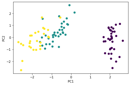
Dimension reduction¶

[54]:

from pyspark.ml.feature import PCA

[55]:

pca = PCA(k=2, inputCol='features', outputCol='pc').fit(train_df_scaled)

[56]:

train_df_scaled = pca.transform(train_df_scaled)

[57]:

train_df_scaled.select('pc').show(5, truncate=False)

+----------------------------------------+
|pc                                      |
+----------------------------------------+
|[2.1719561815281754,0.7342240484007609] |
|[2.3257684348824283,0.11499107410380768]|
|[2.2379887825335114,0.47537636776842684]|
|[1.9410238356438345,0.7700780683206433] |
|[2.0469675488421304,0.5739261085291683] |
+----------------------------------------+
only showing top 5 rows

[58]:

import matplotlib.pyplot as plt

[59]:

pdf = (
    train_df_scaled.select('label', 'pc').
    withColumn("pc", vector_to_array("pc")).
    select(["label"] + [col("pc")[i] for i in range(2)])
).toPandas()

[60]:

pdf.head(3)

[60]:

	pc[0]	pc[1]
0	2.171956	0.734224
1	2.325768	0.114991
2	2.237989	0.475376

[61]:

plt.scatter(pdf.iloc[:, 1], pdf.iloc[:, 2], c=pdf.iloc[:, 0])
plt.xlabel('PC1')
plt.ylabel('PC2')
plt.tight_layout()

../_images/notebooks_C07_Spark_ML_73_0.png

Clustering¶

[62]:

from pyspark.ml.clustering import GaussianMixture

[63]:

gmm = GaussianMixture(
    featuresCol='features',
    k=3,
    seed=0)

[64]:

gmm = gmm.fit(train_df_scaled)

[65]:

gmm.gaussiansDF.toPandas()

[65]:

	mean	cov
0	[-0.9380257346418976, 0.8046671327476248, -1.2...	DenseMatrix([[0.2166823 , 0.29970786, 0.013235...
1	[0.005938775919945091, -0.5221004264901148, 0....	DenseMatrix([[ 0.10356088, -0.0849359 , 0.056...
2	[0.6061006081018865, -0.4609677242002642, 0.72...	DenseMatrix([[0.65443637, 0.40398667, 0.255851...

[66]:

train_df_scaled = gmm.transform(train_df_scaled)

[67]:

train_df_scaled.select('features', 'label', 'probability', 'prediction').sample(0.1).show()

+--------------------+-----+--------------------+----------+
|            features|label|         probability|prediction|
+--------------------+-----+--------------------+----------+
|[-1.5213158492369...|  0.0|[0.99999999999278...|         0|
|[-0.2089130919726...|  1.0|[5.51104734455841...|         1|
|[-0.0776728162462...|  1.0|[6.94499110009014...|         1|
|[0.70976883811231...|  2.0|[9.24177181915992...|         2|
|[2.02217159537659...|  2.0|[2.49896507749226...|         2|
|[0.31604801093303...|  2.0|[6.91948378303032...|         2|
+--------------------+-----+--------------------+----------+

Supervised Learning¶

[68]:

train_df_scaled = train_df_scaled.select('features', 'label')

[69]:

test_df_scaled = test_df_scaled.select('features', 'label')

[70]:

from pyspark.ml.classification import RandomForestClassifier

[71]:

rf = RandomForestClassifier(
    numTrees=10,
    maxDepth=3,
    seed=0
)

[72]:

rf = rf.fit(train_df_scaled)

[73]:

test_df_scaled = rf.transform(test_df_scaled)

[74]:

test_df_scaled.sample(0.1).show()

+--------------------+-----+--------------------+--------------------+----------+
|            features|label|       rawPrediction|         probability|prediction|
+--------------------+-----+--------------------+--------------------+----------+
|[0.31604801093303...|  1.0|[0.03030303030303...|[0.00303030303030...|       1.0|
+--------------------+-----+--------------------+--------------------+----------+

Model evaluation¶

[75]:

from pyspark.ml.evaluation import MulticlassClassificationEvaluator

[76]:

evaluator = MulticlassClassificationEvaluator()

[77]:

evaluator.evaluate(test_df_scaled)

[77]:

0.9618662587412588

[78]:

evaluator = evaluator.setMetricName('accuracy')

[79]:

evaluator.evaluate(test_df_scaled)

[79]:

0.9615384615384616

Pipelines¶

We can assemble pipeline for convenience and reproducibility. This is very similar to what you would do with sklearn, except that MLLib allows you to handle massive datasets by distributing the analysis to multiple computers.

We will put all the preceding steps into the pipeline, and also add hyperparameter optimization via cross-validation.

[80]:

from pyspark.ml import Pipeline

[81]:

from pyspark.ml.tuning import CrossValidator, ParamGridBuilder

[82]:

assembler = VectorAssembler(
    inputCols=iris.columns[:-1],
    outputCol='raw_features'
)
scaler = StandardScaler(
    withMean=True,
    withStd=True,
    inputCol='raw_features',
    outputCol='features'
)
indexer = StringIndexer(
    inputCol="species",
    outputCol="label"
)
rf = RandomForestClassifier()
params = (
    ParamGridBuilder().
    addGrid(rf.numTrees, [5,10,25]).
    addGrid(rf.maxDepth, [3,4,5]).
    build()
)
evaluator = MulticlassClassificationEvaluator(
    metricName='accuracy'
)
cv = CrossValidator(
    estimator=rf,
    evaluator=evaluator,
    estimatorParamMaps=params,
    numFolds=3,
    seed=0
).setParallelism(4)

[83]:

pipeline = Pipeline(
    stages=[assembler, scaler, indexer, cv]
)

[84]:

train_iris, test_iris = iris.randomSplit([2.0, 1.0], seed=0)

[85]:

model = pipeline.fit(train_iris)

[86]:

model.stages

[86]:

[VectorAssembler_b707c6dd0daa,
 StandardScalerModel: uid=StandardScaler_6f905091c141, numFeatures=4, withMean=true, withStd=true,
 StringIndexerModel: uid=StringIndexer_680263d99f3c, handleInvalid=error,
 CrossValidatorModel_a1e2fa6e9d8f]

[87]:

df_cv = pd.DataFrame(list(zip(model.stages[3].getEstimatorParamMaps(), model.stages[3].avgMetrics)))
df_cv[['numTrees', 'maxDepth']] = df_cv[0].apply(lambda x: pd.Series(list(x.values())))
df_cv = df_cv.drop(0, axis=1)
df_cv = df_cv.iloc[:, [1,2,0]]
df_cv.columns = df_cv.columns[:2].tolist() + ['accuracy']
df_cv.sort_values('accuracy', ascending=False)

[87]:

	numTrees	maxDepth	accuracy
6	25	3	0.958970
7	25	4	0.958970
8	25	5	0.958970
5	10	5	0.948217
2	5	5	0.941426
0	5	3	0.940685
3	10	3	0.936723
4	10	4	0.936723
1	5	4	0.929932

[88]:

prediction = model.transform(test_iris)

[89]:

evaluator.evaluate(prediction)

[89]:

0.9807692307692307

Using Spark for non-MLLib models¶

We can also run non-MLLIB machine learning algorithms using Spark.

Hyper-parameter optimization¶

[90]:

! python3 -m pip install --quiet joblibspark

[91]:

from sklearn.svm import SVC
from sklearn.model_selection import train_test_split, GridSearchCV
from sklearn.utils import parallel_backend
from joblibspark import register_spark

[92]:

url = 'https://bit.ly/3eoBK6t'
iris = pd.read_csv(url)

X = iris.iloc[:, :-1]
y = iris.species.astype('category').cat.codes

X_train, X_test, y_train, y_test = train_test_split(X, y)

[93]:

svc = SVC(random_state=0)
params = dict(
    C = [0.1, 1, 10],
    kernel = ['linear', 'poly', 'rbf', 'sigmoid']
)
cv = GridSearchCV(svc, params, cv=3)

[94]:

register_spark()

[95]:

with parallel_backend('spark', n_jobs=4):
    cv.fit(X_train, y_train)

[96]:

pd.DataFrame(cv.cv_results_)

[96]:

	mean_fit_time	std_fit_time	mean_score_time	std_score_time	param_C	param_kernel	params	split0_test_score	split1_test_score	split2_test_score	mean_test_score	std_test_score	rank_test_score
0	0.003228	0.000145	0.002065	0.000645	0.1	linear	{'C': 0.1, 'kernel': 'linear'}	0.973684	0.972973	0.972973	0.973210	0.000335	3
1	0.003249	0.000082	0.001860	0.000418	0.1	poly	{'C': 0.1, 'kernel': 'poly'}	0.973684	0.972973	0.972973	0.973210	0.000335	3
2	0.003456	0.000053	0.001981	0.000424	0.1	rbf	{'C': 0.1, 'kernel': 'rbf'}	0.763158	0.864865	0.756757	0.794927	0.049523	9
3	0.003865	0.000290	0.002149	0.000506	0.1	sigmoid	{'C': 0.1, 'kernel': 'sigmoid'}	0.368421	0.351351	0.351351	0.357041	0.008047	10
4	0.003543	0.000460	0.002302	0.000091	1	linear	{'C': 1, 'kernel': 'linear'}	1.000000	0.972973	0.972973	0.981982	0.012741	1
5	0.003509	0.000452	0.002630	0.000460	1	poly	{'C': 1, 'kernel': 'poly'}	0.947368	0.945946	0.972973	0.955429	0.012419	6
6	0.003940	0.000466	0.002706	0.000336	1	rbf	{'C': 1, 'kernel': 'rbf'}	0.973684	0.972973	0.972973	0.973210	0.000335	3
7	0.004211	0.000627	0.003025	0.000451	1	sigmoid	{'C': 1, 'kernel': 'sigmoid'}	0.368421	0.351351	0.351351	0.357041	0.008047	10
8	0.003760	0.000423	0.002659	0.000333	10	linear	{'C': 10, 'kernel': 'linear'}	0.947368	0.972973	0.918919	0.946420	0.022078	7
9	0.004453	0.000755	0.002508	0.000103	10	poly	{'C': 10, 'kernel': 'poly'}	0.921053	0.972973	0.918919	0.937648	0.024994	8
10	0.004332	0.000757	0.003176	0.000364	10	rbf	{'C': 10, 'kernel': 'rbf'}	1.000000	0.972973	0.972973	0.981982	0.012741	1
11	0.005562	0.000661	0.003428	0.000818	10	sigmoid	{'C': 10, 'kernel': 'sigmoid'}	0.210526	0.297297	0.243243	0.250356	0.035779	12

[97]:

url = 'https://bit.ly/3eoBK6t'
iris = pd.read_csv(url)

X = iris.iloc[:, :-1]
y = iris.species.astype('category').cat.codes

X_train, X_test, y_train, y_test = train_test_split(X, y)

[98]:

n, p = X_train.shape

[99]:

from sklearn.ensemble import RandomForestClassifier
from sklearn.model_selection import cross_val_score

[100]:

import optuna

class Objective(object):
    def __init__(self, X, y):
        self.X = X
        self.y = y

    def __call__(self, trial):
        X, y = self.X, self.y # load data once only

        criterion = trial.suggest_categorical('criterion', ['gini', 'entropy'])
        n_estimators = trial.suggest_int('n_estimators', 50, 201)
        max_features = trial.suggest_float('max_features', 1/p, 1)
        max_depth = trial.suggest_float('max_depth', 1, 128, log=True)
        min_samples_split = trial.suggest_int('min_samples_split', 2, 11, 1)
        min_samples_leaf = trial.suggest_int('min_samples_leaf', 1, 11, 1)

        clf = RandomForestClassifier(
            criterion = criterion,
            n_estimators = n_estimators,
            max_features = max_features,
            max_depth = max_depth,
            min_samples_split = min_samples_split,
            min_samples_leaf = min_samples_leaf,
        )

        score = cross_val_score(clf, X, y,  cv=5).mean()
        return score

objective =  Objective(X_train, y_train)
study = optuna.create_study(direction='maximize', storage='sqlite:///memory')

n_jobs = 4
with parallel_backend('spark', n_jobs=n_jobs):
    study.optimize(objective, n_trials=100, n_jobs=n_jobs)

[I 2020-11-04 12:47:30,511] A new study created in RDB with name: no-name-97aab8f6-8b87-4d03-afe2-5f85415b9671

[101]:

study.trials_dataframe().head(10)

[101]:

	number	value	datetime_start	datetime_complete	duration	params_criterion	params_max_depth	params_max_features	params_min_samples_leaf	params_min_samples_split	params_n_estimators	state
0	0	0.804348	2020-11-04 12:47:31.659174	2020-11-04 12:47:32.204716	0 days 00:00:00.545542	entropy	1.966860	0.457199	9	8	74	COMPLETE
1	1	0.964032	2020-11-04 12:47:31.659435	2020-11-04 12:47:32.745937	0 days 00:00:01.086502	gini	1.792140	0.997070	1	10	147	COMPLETE
2	2	0.955336	2020-11-04 12:47:31.659935	2020-11-04 12:47:32.810389	0 days 00:00:01.150454	entropy	118.759561	0.262684	1	8	146	COMPLETE
3	3	0.964427	2020-11-04 12:47:31.660439	2020-11-04 12:47:32.619121	0 days 00:00:00.958682	gini	4.435854	0.761082	7	4	128	COMPLETE
4	4	0.964427	2020-11-04 12:47:33.254434	2020-11-04 12:47:34.555648	0 days 00:00:01.301214	entropy	15.285156	0.795445	6	10	180	COMPLETE
5	5	0.937154	2020-11-04 12:47:33.691416	2020-11-04 12:47:34.149519	0 days 00:00:00.458103	gini	9.179145	0.301613	10	3	60	COMPLETE
6	6	0.964427	2020-11-04 12:47:33.780986	2020-11-04 12:47:34.522994	0 days 00:00:00.742008	gini	21.264760	0.675328	5	8	102	COMPLETE
7	7	0.964427	2020-11-04 12:47:33.831960	2020-11-04 12:47:34.710602	0 days 00:00:00.878642	gini	4.772650	0.518421	2	9	119	COMPLETE
8	8	0.955336	2020-11-04 12:47:35.174596	2020-11-04 12:47:36.389685	0 days 00:00:01.215089	entropy	30.773008	0.600859	8	5	175	COMPLETE
9	9	0.855336	2020-11-04 12:47:35.531175	2020-11-04 12:47:36.231259	0 days 00:00:00.700084	entropy	1.937602	0.955016	6	10	99	COMPLETE

Using spark with a non-MLLib classifier¶

While there is no easy way to train a general ML model in parallel, we can use Spark for distributed predictions once the model is trained,

[102]:

url = 'https://bit.ly/3eoBK6t'
iris = pd.read_csv(url)

X = iris.iloc[:, :-1]
y = iris.species.astype('category').cat.codes

X_train, X_test, y_train, y_test = train_test_split(X, y)

We use the best parameters found by Optuna in the distributed hyperparameter optimization above.

[103]:

study.best_params

[103]:

{'criterion': 'gini',
 'max_depth': 4.435854141101209,
 'max_features': 0.7610816811817611,
 'min_samples_leaf': 7,
 'min_samples_split': 4,
 'n_estimators': 128}

[104]:

rf = RandomForestClassifier(**study.best_params, random_state=0)

[105]:

rf.fit(X_train, y_train)

[105]:

RandomForestClassifier(max_depth=4.435854141101209,
                       max_features=0.7610816811817611, min_samples_leaf=7,
                       min_samples_split=4, n_estimators=128, random_state=0)

[106]:

from joblib import dump, load

dump(rf, 'rf.joblib')

[106]:

['rf.joblib']

[107]:

def predict(iterartor):
    model = load('rf.joblib') # model is only loaded once
    for features in iterartor:
        yield pd.DataFrame(model.predict(features))

[108]:

df = spark.createDataFrame(X_test)

[109]:

help(df.mapInPandas)

Help on method mapInPandas in module pyspark.sql.pandas.map_ops:

mapInPandas(func, schema) method of pyspark.sql.dataframe.DataFrame instance
    Maps an iterator of batches in the current :class:`DataFrame` using a Python native
    function that takes and outputs a pandas DataFrame, and returns the result as a
    :class:`DataFrame`.

    The function should take an iterator of `pandas.DataFrame`\s and return
    another iterator of `pandas.DataFrame`\s. All columns are passed
    together as an iterator of `pandas.DataFrame`\s to the function and the
    returned iterator of `pandas.DataFrame`\s are combined as a :class:`DataFrame`.
    Each `pandas.DataFrame` size can be controlled by
    `spark.sql.execution.arrow.maxRecordsPerBatch`.

    :param func: a Python native function that takes an iterator of `pandas.DataFrame`\s, and
        outputs an iterator of `pandas.DataFrame`\s.
    :param schema: the return type of the `func` in PySpark. The value can be either a
        :class:`pyspark.sql.types.DataType` object or a DDL-formatted type string.

    >>> from pyspark.sql.functions import pandas_udf
    >>> df = spark.createDataFrame([(1, 21), (2, 30)], ("id", "age"))
    >>> def filter_func(iterator):
    ...     for pdf in iterator:
    ...         yield pdf[pdf.id == 1]
    >>> df.mapInPandas(filter_func, df.schema).show()  # doctest: +SKIP
    +---+---+
    | id|age|
    +---+---+
    |  1| 21|
    +---+---+

    .. seealso:: :meth:`pyspark.sql.functions.pandas_udf`

    .. note:: Experimental

    .. versionadded:: 3.0

[110]:

pred = df.mapInPandas(predict, 'pred double')

[111]:

rf.predict(X_test)[:5]

[111]:

array([2, 1, 1, 1, 1], dtype=int8)

[112]:

pred.show(5)

+----+
|pred|
+----+
| 2.0|
| 1.0|
| 1.0|
| 1.0|
| 1.0|
+----+
only showing top 5 rows

[ ]: