import warnings
warnings.simplefilter('ignore', FutureWarning)
warnings.simplefilter('ignore', UserWarning)

Imbalanced data

Imbalanced data occurs in classification when the number of instances in each class are not the same. Some care is required to learn to predict the rare classes effectively.

There is no one-size-fits-all approach to handling imbalanced data. A reasonable strategy is to consider this as a model selection problem, and use cross-validation to find an approach that works well for your data sets. We will show how to do this in the hyper-parameter optimization notebook.

Warning: Like most things in ML, techniques should not be applied blindly, but considered carefully with the problem goal in mind. In many cases, there is a decision-theoretic problem of assigning the appropriate costs to minority and majority case mistakes that requires domain knowledge to model correctly. As you will see in this example, blind application of a technique does not necessarily improve performance.

Simulate an imbalanced data set

import pandas as pd
import numpy as np

X_train = pd.read_csv('data/X_train.csv')
X_test = pd.read_csv('data/X_test.csv')
y_train = pd.read_csv('data/y_train.csv')
y_test = pd.read_csv('data/y_test.csv')
X = pd.concat([X_train, X_test])
y = pd.concat([y_train, y_test]).squeeze()

y.value_counts()

0    809
1    500
Name: survived, dtype: int64

np.random.seed(0)

idx = (
    (y == 0) |
    ((y == 1) & (np.random.uniform(0, 1, y.shape) < 0.2))
).squeeze()

X_im, y_im = X.loc[idx, :], y[idx]

from sklearn.model_selection import train_test_split

X_train, X_test, y_train, y_test = train_test_split(X_im, y_im, random_state=0)

y_test.value_counts(), y_train.value_counts()

(0    204
 1     25
 Name: survived, dtype: int64,
 0    605
 1     80
 Name: survived, dtype: int64)

Collect more data

This is the best but often impractical solution. Synthetic data generation may also be an option.

Use evaluation metrics that are less sensitive to imbalance

For example, the F1 score (harmonic mean of precision and recall) is less sensitive than the accuracy score.

from sklearn.linear_model import LogisticRegression
from sklearn.utils import class_weight
from sklearn.metrics import roc_auc_score, confusion_matrix

from sklearn.dummy import DummyClassifier

clf = DummyClassifier(strategy='prior')

clf.fit(X_train, y_train)

DummyClassifier(strategy='prior')

clf.score(X_test, y_test)

0.8908296943231441

from sklearn.metrics import accuracy_score, f1_score, balanced_accuracy_score

accuracy_score(clf.predict(X_test), y_test)

0.8908296943231441

f1_score(clf.predict(X_test), y_test)

0.0

lr = LogisticRegression()

lr.fit(X_train, y_train)

LogisticRegression()

accuracy_score(lr.predict(X_test), y_test)

0.9213973799126638

balanced_accuracy_score(lr.predict(X_test), y_test)

0.8723936613844872

f1_score(lr.predict(X_test), y_test)

0.5

Over-sample the minority class

There are many ways to over-sample the minority class. A popular algorithm is known as SMOTE (Synthetic Minority Oversampling Technique)

! python3 -m pip install --quiet imbalanced-learn

import imblearn

X_train_resampled, y_train_resampled = \
imblearn.over_sampling.SMOTE().fit_resample(X_train, y_train)

X_train.shape

(685, 11)

X_train_resampled.shape

(1210, 11)

y_train.value_counts()

0    605
1     80
Name: survived, dtype: int64

Evaluate if this helps

lr = LogisticRegression()

lr.fit(X_train, y_train)

LogisticRegression()

f1_score(lr.predict(X_test), y_test)

0.5

confusion_matrix(lr.predict(X_test), y_test)

array([[202,  16],
       [  2,   9]])

lr.fit(X_train_resampled, y_train_resampled)

LogisticRegression()

f1_score(lr.predict(X_test), y_test)

0.4109589041095891

confusion_matrix(lr.predict(X_test), y_test)

array([[171,  10],
       [ 33,  15]])

Under-sample the majority class

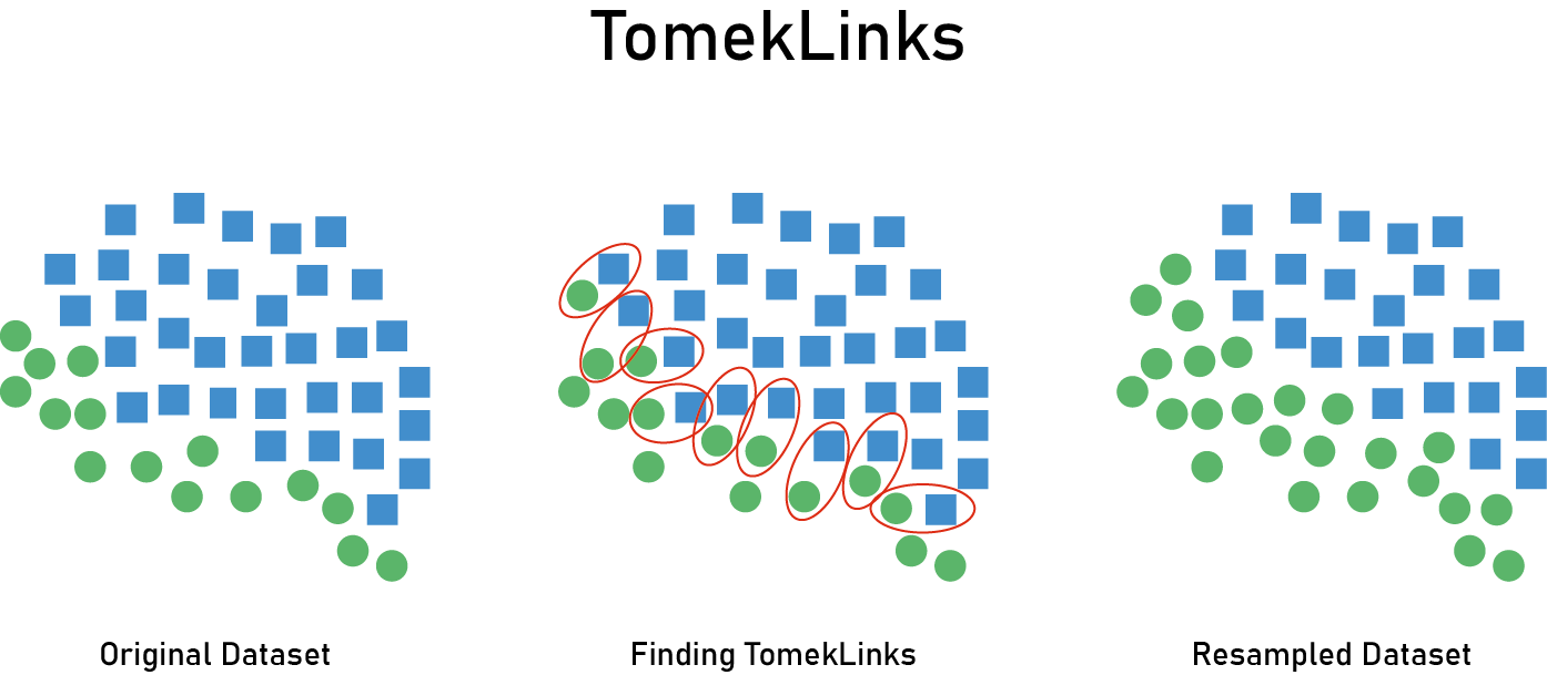
Tomek pairs are nearest neighbor pairs of instances where the classes are different. Under-sampling is done by removing the majority member of the pair.

X_train_resampled, y_train_resampled = \
imblearn.under_sampling.TomekLinks().fit_resample(X_train, y_train)

X_train.shape

(685, 11)

X_train_resampled.shape

(665, 11)

y_train.value_counts()

0    605
1     80
Name: survived, dtype: int64

y_train_resampled.value_counts()

0    585
1     80
Name: survived, dtype: int64

Evaluate if this helps

lr = LogisticRegression()

lr.fit(X_train, y_train)

LogisticRegression()

f1_score(lr.predict(X_test), y_test)

0.5

confusion_matrix(lr.predict(X_test), y_test)

array([[202,  16],
       [  2,   9]])

lr.fit(X_train_resampled, y_train_resampled)

LogisticRegression()

f1_score(lr.predict(X_test), y_test)

0.5

confusion_matrix(lr.predict(X_test), y_test)

array([[202,  16],
       [  2,   9]])

Combine over- and under-sampling

For example, over-sample using SMOTE then clean using Tomek.

X_train_resampled, y_train_resampled = \
imblearn.combine.SMOTETomek().fit_resample(X_train, y_train)

X_train.shape

(685, 11)

X_train_resampled.shape

(1174, 11)

y_train.value_counts()

0    605
1     80
Name: survived, dtype: int64

y_train_resampled.value_counts()

1    587
0    587
Name: survived, dtype: int64

Evaluate if this helps

lr = LogisticRegression()

lr.fit(X_train, y_train)

LogisticRegression()

f1_score(lr.predict(X_test), y_test)

0.5

confusion_matrix(lr.predict(X_test), y_test)

array([[202,  16],
       [  2,   9]])

lr.fit(X_train_resampled, y_train_resampled)

LogisticRegression()

f1_score(lr.predict(X_test), y_test)

0.40540540540540543

confusion_matrix(lr.predict(X_test), y_test)

array([[170,  10],
       [ 34,  15]])

Use class weights to adjust the loss function

We make prediction errors in the minority class more costly than prediction errors in the majority class.

wts = class_weight.compute_class_weight('balanced', np.unique(y_train), y_train)

wts

array([0.5661157, 4.28125  ])

You can then pass in the class weights. Note that there are several alternative ways to calculate possible class weights to use, and you can also do a GridSearch on weights.

This is actually built-in to most classifiers. The defaults are equal weights to each class.

lr = LogisticRegression(class_weight=wts)

lr.fit(X_train, y_train)

LogisticRegression(class_weight=array([0.5661157, 4.28125  ]))

lr.class_weight

array([0.5661157, 4.28125  ])

f1_score(lr.predict(X_test), y_test)

0.5

roc_auc_score(lr.predict(X_test), y_test)

0.8723936613844872

confusion_matrix(lr.predict(X_test), y_test)

array([[202,  16],
       [  2,   9]])

lr_balanced = LogisticRegression(class_weight='balabced')

lr_balanced.class_weight

'balabced'

lr_balanced.fit(X_train, y_train)

LogisticRegression(class_weight='balabced')

roc_auc_score(lr_balanced.predict(X_test), y_test)

0.8723936613844872

confusion_matrix(lr_balanced.predict(X_test), y_test)

array([[202,  16],
       [  2,   9]])

f1_score(lr_balanced.predict(X_test), y_test)

0.5

Use a classifier that is less sensitive to imbalance

Boosted trees are generally good because of their sequential nature.

from catboost import CatBoostClassifier

cb = CatBoostClassifier()

cb.fit(X_train, y_train, verbose=0)

<catboost.core.CatBoostClassifier at 0x135202880>

f1_score(cb.predict(X_test), y_test)

0.5263157894736842

confusion_matrix(cb.predict(X_test), y_test)

array([[201,  15],
       [  3,  10]])

Imbalanced learn has classifiers that balance the data automatically

from imblearn.ensemble import BalancedRandomForestClassifier

brf = BalancedRandomForestClassifier()

brf.fit(X_train, y_train)

BalancedRandomForestClassifier()

confusion_matrix(brf.predict(X_test), y_test)

array([[154,   8],
       [ 50,  17]])

f1_score(brf.predict(X_test), y_test)

0.3695652173913044