Deep Learning Models¶

This is not a deep learning course, but by request, I will introduce simple examples to get started in deep learning and highlight some aspects that I find interesting. In particular, strategies for optimization and specialized architectures are not covered.

Note: This is a version for those of you on a Mac with AMD GPU - we can use the PlaidML backend to take advantage of the GPU. Note that this works with the standalone keras, not the tensorflow version.

First install

python3 -m pip install -U --quiet plaidml-keras plaidbench

Then run and choose the GPU as default device

plaidml-setup

[1]:

import os
os.environ['KERAS_BACKEND'] = 'plaidml.keras.backend'
os.environ['RUNFILES_DIR'] = '/usr/local/share/plaidml'
os.environ['PLAIDML_NATIVE_PATH'] = '/usr/local/lib/libplaidml.dylib'

[2]:

%matplotlib inline

[3]:

import warnings
warnings.simplefilter('ignore', RuntimeWarning)

[4]:

import matplotlib.pyplot as plt
import pandas as pd
import numpy as np
import seaborn as sns

[5]:

import tensorflow as tf
import keras

Using plaidml.keras.backend backend.

[6]:

from keras.utils import plot_model

[7]:

import tensorflow_datasets as tfds

Building models¶

Prepare data¶

[8]:

import seaborn as sns

[9]:

iris = sns.load_dataset('iris')
iris.species = iris.species.astype('category').cat.codes
iris = iris.sample(frac=1)

[10]:

X_train, y_train = iris.iloc[:, :-1].values, iris.iloc[:, -1].values

[11]:

X_train = X_train.astype('float32')

Pre-process data¶

If you need to pre-process your data, see https://keras.io/api/preprocessing/. We will not do any pre-processing for simplicity.

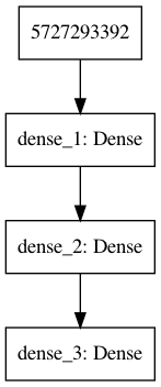
Sequential API¶

If the entire pipeline is a single chain of layers, the Sequential API is the simplest to use.

[12]:

from keras.models import Sequential, Model
from keras.layers import Dense, Input, concatenate

Set random seed for reproducibility¶

[13]:

np.random.seed(0)
tf.random.set_seed(0)

[14]:

X_train[0].shape

[14]:

(4,)

[15]:

model = Sequential()
model.add(Dense(8, input_shape=X_train[0].shape))
model.add(Dense(4, activation='relu'))
model.add(Dense(3, activation='softmax'))

INFO:plaidml:Opening device "metal_amd_radeon_pro_560x.0"

Alternative model specification

model = Sequential(
    Dense(8, input_shape=(4,)),
    Dense(4, activation='relu'),
    Dense(3, activation='softmax')
)

[16]:

model.compile(
    optimizer='adam',
    loss='sparse_categorical_crossentropy',
    metrics=['accuracy']
)

[17]:

model.summary()

_________________________________________________________________
Layer (type)                 Output Shape              Param #
=================================================================
dense_1 (Dense)              (None, 8)                 40
_________________________________________________________________
dense_2 (Dense)              (None, 4)                 36
_________________________________________________________________
dense_3 (Dense)              (None, 3)                 15
=================================================================
Total params: 91
Trainable params: 91
Non-trainable params: 0
_________________________________________________________________

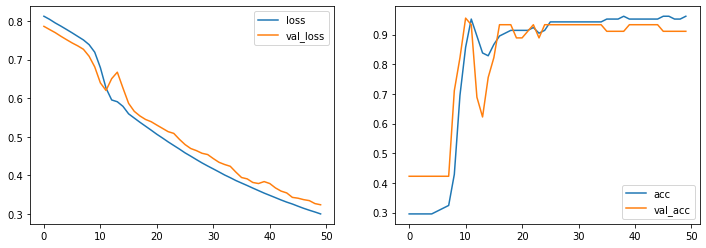
[18]:

hist = model.fit(
    X_train,
    y_train,
    validation_split = 0.3,
    epochs=50,
    verbose=0)

[19]:

fig, axes = plt.subplots(1,2,figsize=(12, 4))
for ax, measure in zip(axes, ['loss', 'acc']):
    ax.plot(hist.history[measure], label=measure)
    ax.plot(hist.history['val_' + measure], label='val_' + measure)
    ax.legend()
pass

../_images/notebooks_B13_Deep_Learning_Models_PlaidML_26_0.png

[20]:

plot_model(model)

[21]:

from IPython.display import Image

[22]:

Image('model.png')

[22]:

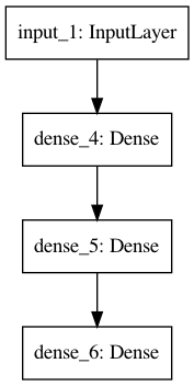
../_images/notebooks_B13_Deep_Learning_Models_PlaidML_29_0.png

Functional API¶

The functional API provides flexibility, allowing you to build models with multiple inputs, multiple outputs, or branch and merge architectures.

Set random seed for reproducibility¶

[23]:

np.random.seed(0)
tf.random.set_seed(0)

[24]:

input = Input(shape=(4,))
x = Dense(8)(input)
x = Dense(4, activation='relu')(x)
output = Dense(3, activation='softmax')(x)
model = Model(inputs=[input], outputs=[output])

[25]:

model.compile(
    optimizer='adam',
    loss='sparse_categorical_crossentropy',
    metrics=['accuracy']
)

[26]:

model.summary()

_________________________________________________________________
Layer (type)                 Output Shape              Param #
=================================================================
input_1 (InputLayer)         (None, 4)                 0
_________________________________________________________________
dense_4 (Dense)              (None, 8)                 40
_________________________________________________________________
dense_5 (Dense)              (None, 4)                 36
_________________________________________________________________
dense_6 (Dense)              (None, 3)                 15
=================================================================
Total params: 91
Trainable params: 91
Non-trainable params: 0
_________________________________________________________________

[27]:

hist = model.fit(
    X_train,
    y_train,
    validation_split = 0.3,
    epochs=50,
    verbose=0)

[28]:

fig, axes = plt.subplots(1,2,figsize=(12, 4))
for ax, measure in zip(axes, ['loss', 'acc']):
    ax.plot(hist.history[measure], label=measure)
    ax.plot(hist.history['val_' + measure], label='val_' + measure)
    ax.legend()
pass

../_images/notebooks_B13_Deep_Learning_Models_PlaidML_37_0.png

[29]:

plot_model(model)
Image('model.png')

[29]:

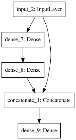
../_images/notebooks_B13_Deep_Learning_Models_PlaidML_38_0.png

Flexibility of functional API¶

You can easily implement multiple inputs, multiple outputs or skip connections. Note that if you have multiple outputs, you probably also want multiple loss functions given as a list in the compile step (unless the same loss function is applicable to both outputs).

[30]:

input = Input(shape=(4,))
x1 = Dense(8)(input)
x2 = Dense(4, activation='relu')(x1)
x3 = concatenate([input, x2])
output = Dense(3, activation='softmax')(x3)
model = Model(inputs=[input], outputs=[output])

[31]:

plot_model(model)
Image('model.png')

[31]:

../_images/notebooks_B13_Deep_Learning_Models_PlaidML_41_0.png

Hyperparameter optimization¶

[32]:

import optuna

[33]:

from keras.layers import Conv2D, MaxPooling2D, Dropout, Flatten

[34]:

(X_train, y_train), (X_test, y_test) = tf.keras.datasets.mnist.load_data()
X_train, X_test = X_train / 255.0, X_test / 255.0
X_train = X_train.astype('float32')
X_test = X_test.astype('float32')
X_train = X_train.reshape(X_train.shape[0], 28, 28, 1)
X_test = X_test.reshape(X_test.shape[0], 28, 28, 1)

[35]:

class Objective(object):
    def __init__(self, X, y,
                 max_epochs,
                 input_shape,
                 num_classes):
        self.X = X
        self.y = y
        self.max_epochs = max_epochs
        self.input_shape = input_shape
        self.num_classes = num_classes

    def __call__(self, trial):
        dropout=trial.suggest_discrete_uniform('dropout', 0.05, 0.5, 0.05)
        batch_size = trial.suggest_categorical('batch_size', [32, 64, 96, 128])

        params = dict(
            dropout = dropout,
            batch_size = batch_size
        )

        model = Sequential()
        model.add(Conv2D(32, kernel_size=(3, 3),
                         activation='relu',
                         input_shape=self.input_shape))
        model.add(Conv2D(64, (3, 3), activation='relu'))
        model.add(MaxPooling2D(pool_size=(2, 2)))
        model.add(Dropout(params['dropout']))
        model.add(Flatten())
        model.add(Dense(128, activation='relu'))
        model.add(Dropout(params['dropout']))
        model.add(Dense(self.num_classes, activation='softmax'))

        model.compile(optimizer='adam',
                      loss='sparse_categorical_crossentropy',
                      metrics=['accuracy'])

        # fit the model
        hist = model.fit(x=self.X, y=self.y,
                          batch_size=params['batch_size'],
                          validation_split=0.25,
                          epochs=self.max_epochs)

        loss = np.min(hist.history['val_loss'])

        return loss

[36]:

optuna.logging.set_verbosity(0)

[37]:

N = 5
max_epochs = 3
input_shape = (28,28,1)
num_classes = 10

[38]:

%%time

objective1 = Objective(X_train, y_train, max_epochs, input_shape, num_classes)
study1 = optuna.create_study(direction='minimize')
study1.optimize(objective1, n_trials=N)

Train on 45000 samples, validate on 15000 samples
Epoch 1/3
45000/45000 [==============================] - 19s 430us/step - loss: 0.2965 - acc: 0.9088 - val_loss: 0.0837 - val_acc: 0.9749
Epoch 2/3
45000/45000 [==============================] - 19s 420us/step - loss: 0.1083 - acc: 0.9680 - val_loss: 0.0569 - val_acc: 0.9825
Epoch 3/3
45000/45000 [==============================] - 19s 415us/step - loss: 0.0829 - acc: 0.9752 - val_loss: 0.0493 - val_acc: 0.9859
Train on 45000 samples, validate on 15000 samples
Epoch 1/3
45000/45000 [==============================] - 23s 504us/step - loss: 0.2049 - acc: 0.9371 - val_loss: 0.0688 - val_acc: 0.9793
Epoch 2/3
45000/45000 [==============================] - 19s 423us/step - loss: 0.0540 - acc: 0.9838 - val_loss: 0.0469 - val_acc: 0.9861
Epoch 3/3
45000/45000 [==============================] - 19s 418us/step - loss: 0.0357 - acc: 0.9887 - val_loss: 0.0511 - val_acc: 0.9844
Train on 45000 samples, validate on 15000 samples
Epoch 1/3
45000/45000 [==============================] - 25s 554us/step - loss: 0.1936 - acc: 0.9414 - val_loss: 0.0704 - val_acc: 0.9783
Epoch 2/3
45000/45000 [==============================] - 20s 445us/step - loss: 0.0556 - acc: 0.9826 - val_loss: 0.0522 - val_acc: 0.9836
Epoch 3/3
45000/45000 [==============================] - 20s 446us/step - loss: 0.0366 - acc: 0.9883 - val_loss: 0.0544 - val_acc: 0.9829
Train on 45000 samples, validate on 15000 samples
Epoch 1/3
45000/45000 [==============================] - 23s 511us/step - loss: 0.2214 - acc: 0.9320 - val_loss: 0.0740 - val_acc: 0.9771
Epoch 2/3
45000/45000 [==============================] - 19s 417us/step - loss: 0.0639 - acc: 0.9811 - val_loss: 0.0544 - val_acc: 0.9835
Epoch 3/3
45000/45000 [==============================] - 19s 419us/step - loss: 0.0426 - acc: 0.9870 - val_loss: 0.0446 - val_acc: 0.9866
Train on 45000 samples, validate on 15000 samples
Epoch 1/3
45000/45000 [==============================] - 29s 638us/step - loss: 0.2372 - acc: 0.9277 - val_loss: 0.0643 - val_acc: 0.9809
Epoch 2/3
45000/45000 [==============================] - 22s 498us/step - loss: 0.0898 - acc: 0.9722 - val_loss: 0.0489 - val_acc: 0.9865
Epoch 3/3
45000/45000 [==============================] - 22s 499us/step - loss: 0.0671 - acc: 0.9795 - val_loss: 0.0430 - val_acc: 0.9879
CPU times: user 1min 10s, sys: 1min 11s, total: 2min 22s
Wall time: 5min 16s

[40]:

df = study1.trials_dataframe()

[41]:

df.head()

[41]:

	number	value	datetime_start	datetime_complete	duration	params_batch_size	params_dropout	state
0	0	0.049347	2020-10-21 08:34:48.712812	2020-10-21 08:35:45.753741	0 days 00:00:57.040929	128	0.50	COMPLETE
1	1	0.046897	2020-10-21 08:35:45.753777	2020-10-21 08:36:46.349771	0 days 00:01:00.595994	128	0.15	COMPLETE
2	2	0.052158	2020-10-21 08:36:46.349811	2020-10-21 08:37:51.400444	0 days 00:01:05.050633	96	0.15	COMPLETE
3	3	0.044622	2020-10-21 08:37:51.400485	2020-10-21 08:38:52.037658	0 days 00:01:00.637173	128	0.20	COMPLETE
4	4	0.043021	2020-10-21 08:38:52.037701	2020-10-21 08:40:05.707299	0 days 00:01:13.669598	64	0.45	COMPLETE

[42]:

from optuna.visualization import plot_param_importances

[44]:

plot_param_importances(study1)