Spark Low Level API

Outline

• Foundations

  • Functional programming (Spark RDDs)

  • Use of pandas (Spark DataFramej

  • Use of SQL (Spark SQL)

• Catalyst optimizer

  • Analysis

    • DataFrame

    • SQL AST

  • Logical plan

    • Catalog resolution of names

    • Rule-based optimization

      • Boolean simplification

      • Predicate pushdown

      • Constant folding

      • Projection pruning

  • Physical plan

    • Convert to RDD

    • Cost-based optimization

  • Code generation

    • Project Tungsten

    • Performs role of compiler

    • Generates Java bytecode

Resilient distributed datasets (RDD) - In-memory distributed collections - Removes need to write to disk for fault tolerance - Resilience - Reconstruct from lineage - Immutable - Distributed - RDD data live in one or more partitions - Dataset - Consists of records - Each partition consists of distinct set of records that can be operated on independently - Shared nothing philosophy

• Loading data into RDDs

  • Programmatically

    • range()

    • parallelize()

  • From file

    • Compression

      • Splittable and non-splittable formats

      • Non-splittable files cannot be distributed

      • Splittable formats - LZO, Snappy

      • Non-splittable formats - gzip, zip

    • Data locality

      • Worker partitions from nearby DFS partitions

      • Default partition size is 128 MB

      • Local file system

      • Networked filesystem

      • Distributed filesystem

    • textFile()

    • WoleTextFiles()

  • From data resource

  • From stream

• Persistence

  • persist)

  • cache()

• Types of RDDs

  • Base RDD

  • Pair RDD

  • Double RDD

  • Many others

Base RDD

• Narrow transformations

  • map()

  • filter()

  • flatMap(j

  • distinct()

• Broad transformations

  • reduce()

  • groupby()

  • sortBy()

  • join()

• Actions

  • count()

  • take()

  • takeOrdered()

  • top()

  • collect()

  • saveAsTextFile()

  • first()

  • reduce()

  • fold()

  • aggregate()

  • foreach()

PairedRDD

• Dictionary functions

  • keys()

  • values()

  • keyBy()

• Functional transformations

  • mapValues()

  • flatMapValues()

• Grouping, sorting and aggregation

  • groupByKey()

  • reduceByKey()

  • foldByKey()

  • sortByKey()

• Joins

  • Join large by small

  • join()

  • leftOuterJoin()

  • rightOuterJoin()

  • fullOuterJoin()

  • cogroup()

  • cartesian()

• Set operations

  • union()

  • intersection(j

  • subtract()

  • subtractByKey()

Numeric RDD

• min()

• max()

• sum()

• mean()

• stdev()

• variance()

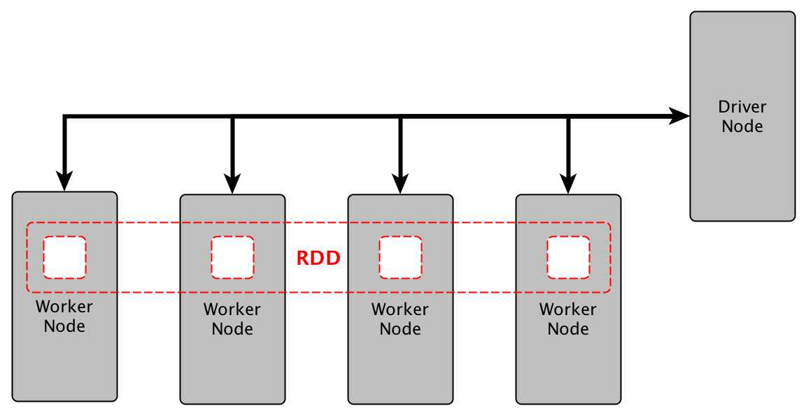
Architecture of a Spark Application

Big picture

You will type your commands iin a local Spark session, and the SparkContext will take care of running your instructions distributed across the workers (executors) on a cluster. Each executor can have 1 or more CPU cores, its own memory cahe, and is responsible for handling its own distributed tasks. Communicaiton between local and workers and between worker and worker is handled by a cluster manager.

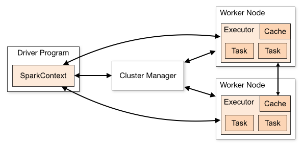
Source: http://spark.apache.org/docs/latest/img/cluster-overview.png

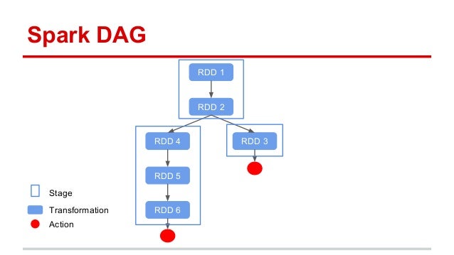
Organizaiton of Spark tasks

Spark organizes tasks that can be performed without exchanging data across partitions into stages. The sequecne of tasks to be perfomed are laid out as a Directed Acyclic Graph (DAG). Tasks are differenitated into transforms (lazy evalutation - just add to DAG) and actions (eager evaluation - execute the specified path in the DAG). Note that calculations are not cached unless requested. Hence if you have triggered the action after RDD3 in the figure, then trigger the aciton after RDD6, RDD2 will be re-generated from RDD1 twice. We can avoid the re-calculation by persisting or cacheing RDD2.

Source: https://image.slidesharecdn.com/mapreducevsspark-150512052504-lva1-app6891/95/map-reduce-vs-spark-16-638.jpg?cb=1431408380

• PySpark API

SparkContext

A SparkContext represents the connection to a Spark cluster, and can be used to create RDDs, accumulators and broadcast variables on that cluster. Here we set it up to use local nodes - the argument locals[*] means to use the local machine as the cluster, using as many worker threads as there are cores. You can also explicitly set the number of cores with locals[k] where k is an integer.

With Saprk 2.0 onwards, there is also a SparkSession that manages DataFrames, which is the preferred abstraction for working in Spark. However DataFrames are composed of RDDs, and it is still necesaary to understand how to use and mainpulate RDDs for low level operations.

Depending on your setup, you many have to import SparkContext. This is not necessary in our Docker containers as we will be using livy.

Start spark

from pyspark import SparkContext
sc =  SparkContext.getOrCreate()

from pyspark.sql import SparkSession
spark = (
    SparkSession.builder
    .master("local")
    .appName("BIOS-823")
    .config("spark.executor.cores", 4)
    .getOrCreate()
)

Use this instead if using Spark on vm-manage containers.

%%spark

import numpy as np

Version

sc.version

'3.0.1'

Number of workers

sc.defaultParallelism

12

Data in an RDD is distributed across partitions. It is most efficient if data does not have to be transferred across partitions. We can see the default minimumn number of partitions, and the actual number in an RDD later.

sc.defaultMinPartitions

2

Resilient Distributed Datasets (RDD)

Creating an RDD

The RDD (Resilient Distributed Dataset) is a data storage abstraction - you can work with it as though it were single unit, while it may actually be distributed over many nodes in the computing cluster.

A first example

Distribute the data set to the workers

xs = sc.parallelize(range(10))
xs

PythonRDD[1] at RDD at PythonRDD.scala:53

xs.getNumPartitions()

12

Return all data within each partition as a list. Note that the glom() operation operates on the distributed workers without centralizing the data.

xs.glom().collect()

[[], [0], [1], [2], [3], [4], [], [5], [6], [7], [8], [9]]

Only keep even numbers

xs = xs.filter(lambda x: x % 2 == 0)
xs

PythonRDD[3] at RDD at PythonRDD.scala:53

Square all elements

xs = xs.map(lambda x: x**2)
xs

PythonRDD[4] at RDD at PythonRDD.scala:53

Execute the code and return the final dataset

xs.collect()

[0, 4, 16, 36, 64]

Reduce also triggers a calculation

xs.reduce(lambda x, y: x+y)

120

A common Spark idiom chains mutiple functions together

(
    sc.parallelize(range(10))
    .filter(lambda x: x % 2 == 0)
    .map(lambda x: x**2)
    .collect()
)

[0, 4, 16, 36, 64]

Actions and transforms

A transform maps an RDD to another RDD - it is a lazy operation. To actually perform any work, we need to apply an action.

Actions

x = sc.parallelize(np.random.randint(1, 6, 10))

x.collect()

[3, 1, 1, 2, 2, 5, 3, 2, 5, 2]

x.take(5)

[3, 1, 1, 2, 2]

x.first()

3

x.top(5)

[5, 5, 3, 3, 2]

x.takeSample(True, 15)

[1, 3, 1, 2, 3, 2, 2, 2, 1, 2, 3, 2, 3, 5, 5]

x.count()

10

x.distinct().collect()

[1, 2, 3, 5]

x.countByValue()

defaultdict(int, {3: 2, 1: 2, 2: 4, 5: 2})

x.sum()

26

x.max()

5

x.mean()

2.6

x.stats()

(count: 10, mean: 2.6, stdev: 1.3564659966250538, max: 5.0, min: 1.0)

Reduce, fold and aggregate actions

From the API:

• reduce(f)

Reduces the elements of this RDD using the specified commutative and associative binary operator. Currently reduces partitions locally.

• fold(zeroValue, op)

Aggregate the elements of each partition, and then the results for all the partitions, using a given associative function and a neutral “zero value.”

The function op(t1, t2) is allowed to modify t1 and return it as its result value to avoid object allocation; however, it should not modify t2.

This behaves somewhat differently from fold operations implemented for non-distributed collections in functional languages like Scala. This fold operation may be applied to partitions individually, and then fold those results into the final result, rather than apply the fold to each element sequentially in some defined ordering. For functions that are not commutative, the result may differ from that of a fold applied to a non-distributed collection.

• aggregate(zeroValue, seqOp, combOp)

Aggregate the elements of each partition, and then the results for all the partitions, using a given combine functions and a neutral “zero value.”

The functions op(t1, t2) is allowed to modify t1 and return it as its result value to avoid object allocation; however, it should not modify t2.

The first function (seqOp) can return a different result type, U, than the type of this RDD. Thus, we need one operation for merging a T into an U and one operation for merging two U

Notes:

• All 3 operations take a binary op with signature op(accumulator, operand)

x = sc.parallelize(np.random.randint(1, 10, 12))

x.collect()

[2, 3, 2, 3, 3, 2, 9, 4, 5, 6, 4, 4]

max using reduce

x.reduce(lambda x, y: x if x > y else y)

9

sum using reduce

x.reduce(lambda x, y: x+y)

47

sum using fold

x.fold(0, lambda x, y: x+y)

47

prod using reduce

x.reduce(lambda x, y: x*y)

3732480

prod using fold

x.fold(1, lambda x, y: x*y)

3732480

sum using aggregate

x.aggregate(0, lambda x, y: x + y, lambda x, y: x + y)

47

count using aggregate

x.aggregate(0, lambda acc, _: acc + 1, lambda x, y: x+y)

12

mean using aggregate

sum_count = x.aggregate([0,0],
                        lambda acc, x: (acc[0]+x, acc[1]+1),
                        lambda acc1, acc2: (acc1[0] + acc2[0], acc1[1]+ acc2[1]))
sum_count[0]/sum_count[1]

3.9166666666666665

Warning: Be very careful with fold and aggregate - the zero value must be “neutral”. The behavior can be different from Python’s reduce with an initial value.

This is because there are two levels of operations that use the zero value - first locally, then globally.

xs = x.collect()

xs = np.array(xs)

xs

array([2, 3, 2, 3, 3, 2, 9, 4, 5, 6, 4, 4])

sum(xs)

47

Exercise: Explain the results shown below:

from functools import reduce

reduce(lambda x, y: x + y, xs, 1)

48

x.fold(1, lambda acc, val: acc + val)

60

x.aggregate(1, lambda x, y: x + y, lambda x, y: x + y)

60

Exercise: Explain the results shown below:

reduce(lambda x, y: x + y**2, xs, 0)

229

np.sum(xs**2)

229

x.fold(0, lambda x, y: x + y**2)

9541

x.aggregate(0, lambda x, y: x + y**2, lambda x, y: x + y)

229

Exercise: Explain the results shown belwo:

x.fold([], lambda acc, val: acc + [val])

[[2], [3], [2], [3], [3], [2], [9], [4], [5], [6], [4], [4]]

seqOp = lambda acc, val: acc + [val]
combOp = lambda acc, val: acc + val
x.aggregate([], seqOp, combOp)

[2, 3, 2, 3, 3, 2, 9, 4, 5, 6, 4, 4]

Transforms

x = sc.parallelize([1,2,3,4])
y = sc.parallelize([3,3,4,6])

x.map(lambda x: x + 1).collect()

[2, 3, 4, 5]

x.filter(lambda x: x%3 == 0).collect()

[3]

Think of flatMap as a map followed by a flatten operation

x.flatMap(lambda x: range(x-2, x)).collect()

[-1, 0, 0, 1, 1, 2, 2, 3]

x.sample(False, 0.5).collect()

[2, 3, 4]

Set-like transformss

y.distinct().collect()

[3, 4, 6]

x.union(y).collect()

[1, 2, 3, 4, 3, 3, 4, 6]

x.intersection(y).collect()

[3, 4]

x.subtract(y).collect()

[1, 2]

x.cartesian(y).collect()

[(1, 3),
 (1, 3),
 (1, 4),
 (1, 6),
 (2, 3),
 (2, 3),
 (2, 4),
 (2, 6),
 (3, 3),
 (3, 3),
 (3, 4),
 (3, 6),
 (4, 3),
 (4, 3),
 (4, 4),
 (4, 6)]

Note that flatmap gets rid of empty lists, and is a good way to ignore “missing” or “malformed” entires.

def conv(x):
    try:
        return [float(x)]
    except:
        return []

s = "Thee square root of 3 is less than 3.14 unless you divide by 0".split()
x = sc.parallelize(s)

x.collect()

['Thee',
 'square',
 'root',
 'of',
 '3',
 'is',
 'less',
 'than',
 '3.14',
 'unless',
 'you',
 'divide',
 'by',
 '0']

x.map(conv).collect()

[[], [], [], [], [3.0], [], [], [], [3.14], [], [], [], [], [0.0]]

x.flatMap(conv).collect()

[3.0, 3.14, 0.0]

Working with key-value pairs

RDDs consissting of key-value pairs are required for many Spark operatinos. They can be created by using a function that returns an RDD composed of tuples.

data = [('ann', 'spring', 'math', 98),
        ('ann', 'fall', 'bio', 50),
        ('bob', 'spring', 'stats', 100),
        ('bob', 'fall', 'stats', 92),
        ('bob', 'summer', 'stats', 100),
        ('charles', 'spring', 'stats', 88),
        ('charles', 'fall', 'bio', 100)
       ]

rdd = sc.parallelize(data)

rdd.keys().collect()

['ann', 'ann', 'bob', 'bob', 'bob', 'charles', 'charles']

rdd.collect()

[('ann', 'spring', 'math', 98),
 ('ann', 'fall', 'bio', 50),
 ('bob', 'spring', 'stats', 100),
 ('bob', 'fall', 'stats', 92),
 ('bob', 'summer', 'stats', 100),
 ('charles', 'spring', 'stats', 88),
 ('charles', 'fall', 'bio', 100)]

Sum values by key

(
    rdd.
    map(lambda x: (x[0], x[3])).
    reduceByKey(lambda x, y: x + y).
    collect()
)

[('charles', 188), ('ann', 148), ('bob', 292)]

Running list of values by key

(
    rdd.
    map(lambda x: ((x[0], x[3]))).
    aggregateByKey([], lambda x, y: x + [y], lambda x, y: x + y).
    collect()
)

[('charles', [88, 100]), ('ann', [98, 50]), ('bob', [100, 92, 100])]

Average by key

(
    rdd.
    map(lambda x: ((x[0], x[3]))).
    aggregateByKey([], lambda x, y: x + [y], lambda x, y: x + y).
    map(lambda x: (x[0], sum(x[1])/len(x[1]))).
    collect()
)

[('charles', 94.0), ('ann', 74.0), ('bob', 97.33333333333333)]

Using a different key

(
    rdd.
    map(lambda x: ((x[2], x[3]))).
    aggregateByKey([], lambda x, y: x + [y], lambda x, y: x + y).
    map(lambda x: (x[0], sum(x[1])/len(x[1]))).
    collect()
)

[('bio', 75.0), ('math', 98.0), ('stats', 95.0)]

Using key-value pairs to find most frequent words in Ulysses

Note: This part assumes that there we are using HDFS.

If you want to install locally, there are tutorials on the web. For Macbook I followed this guide.

hadoop = sc._jvm.org.apache.hadoop

fs = hadoop.fs.FileSystem
conf = hadoop.conf.Configuration()
path = hadoop.fs.Path('./data/texts')

for f in fs.get(conf).listStatus(path):
    print(f.getPath())

hdfs://localhost:9000/user/cliburnchan/data/texts/Portrait.txt
hdfs://localhost:9000/user/cliburnchan/data/texts/Ulysses.txt
hdfs://localhost:9000/user/cliburnchan/data/texts/looking_glass.txt

ulysses = sc.textFile('./data/texts/Portrait.txt')

Note that we can also read in entire docs as the values.

docs = sc.wholeTextFiles('./data/texts/')
docs.keys().collect()

['hdfs://localhost:9000/user/cliburnchan/data/texts/Portrait.txt',
 'hdfs://localhost:9000/user/cliburnchan/data/texts/Ulysses.txt',
 'hdfs://localhost:9000/user/cliburnchan/data/texts/looking_glass.txt']

ulysses.take(10)

["Project Gutenberg's A Portrait of the Artist as a Young Man, by James Joyce",
 '',
 'This eBook is for the use of anyone anywhere at no cost and with',
 'almost no restrictions whatsoever.  You may copy it, give it away or',
 're-use it under the terms of the Project Gutenberg License included',
 'with this eBook or online at www.gutenberg.net',
 '',
 '',
 'Title: A Portrait of the Artist as a Young Man',
 '']

import string
def tokenize(line):
    table = dict.fromkeys(map(ord, string.punctuation))
    return line.translate(table).lower().split()

words = ulysses.flatMap(lambda line: tokenize(line))
words.take(10)

['project',
 'gutenbergs',
 'a',
 'portrait',
 'of',
 'the',
 'artist',
 'as',
 'a',
 'young']

words = words.map(lambda x: (x, 1))
words.take(10)

[('project', 1),
 ('gutenbergs', 1),
 ('a', 1),
 ('portrait', 1),
 ('of', 1),
 ('the', 1),
 ('artist', 1),
 ('as', 1),
 ('a', 1),
 ('young', 1)]

counts = words.reduceByKey(lambda x, y: x+y)
counts.take(10)

[('project', 87),
 ('portrait', 6),
 ('of', 3268),
 ('artist', 18),
 ('as', 484),
 ('young', 53),
 ('james', 5),
 ('this', 216),
 ('ebook', 10),
 ('is', 470)]

counts.takeOrdered(10, key=lambda x: -x[1])

[('the', 6082),
 ('and', 3439),
 ('of', 3268),
 ('a', 2009),
 ('to', 2008),
 ('he', 1854),
 ('his', 1743),
 ('in', 1592),
 ('was', 1067),
 ('that', 961)]

Word count chained version

(
ulysses.flatMap(lambda line: tokenize(line))
                .map(lambda word: (word, 1))
               .reduceByKey(lambda x, y: x + y)
               .takeOrdered(10, key=lambda x: -x[1])
)

[('the', 6082),
 ('and', 3439),
 ('of', 3268),
 ('a', 2009),
 ('to', 2008),
 ('he', 1854),
 ('his', 1743),
 ('in', 1592),
 ('was', 1067),
 ('that', 961)]

Avoiding slow Python UDF tokenize

We will see how to to this in the DataFrames notebook.

CountByValue Action

If you are sure that the results will fit into memory, you can get a dacitonary of counts more easily.

wc = (
    ulysses.
    flatMap(lambda line: tokenize(line)).
    countByValue()
)

wc['the']

6082

Persisting data

The top_word program will repeat ALL the computations each time we take an action such as takeOrdered. We need to persist or cache the results - they are similar except that persist gives more control over how the data is retained.

counts.is_cached

False

counts.persist()

PythonRDD[117] at RDD at PythonRDD.scala:53

counts.is_cached

True

counts.takeOrdered(5, lambda x: -x[1])

[('the', 6082), ('and', 3439), ('of', 3268), ('a', 2009), ('to', 2008)]

counts.take(5)

[('project', 87), ('portrait', 6), ('of', 3268), ('artist', 18), ('as', 484)]

counts.takeOrdered(5, lambda x: x[0])

[('1', 7), ('10', 1), ('11', 1), ('13', 1), ('14', 1)]

counts.keys().take(5)

['project', 'portrait', 'of', 'artist', 'as']

counts.values().take(5)

[87, 6, 3268, 18, 484]

count_dict = counts.collectAsMap()
count_dict['circle']

1

counts.unpersist()

PythonRDD[117] at RDD at PythonRDD.scala:53

counts.is_cached

False

counts.cache()

PythonRDD[117] at RDD at PythonRDD.scala:53

counts.is_cached

True

Merging key, value datasets

We will build a second counts key: value RDD from another of Joyce’s works - Portrait of the Artist as a Young Man.

portrait = sc.textFile('./data/texts/Portrait.txt')

counts1 = (
portrait.flatMap(lambda line: tokenize(line))
        .map(lambda x: (x, 1))
        .reduceByKey(lambda x,y: x+y)
)

counts1.persist()

PythonRDD[129] at RDD at PythonRDD.scala:53

Combine counts for words found in both books

joined = counts.join(counts1)

joined.take(5)

[('project', (87, 87)),
 ('portrait', (6, 6)),
 ('of', (3268, 3268)),
 ('artist', (18, 18)),
 ('as', (484, 484))]

sum counts over words

s = joined.mapValues(lambda x: x[0] + x[1])
s.take(5)

[('project', 174), ('portrait', 12), ('of', 6536), ('artist', 36), ('as', 968)]

average counts across books

avg = joined.mapValues(lambda x: np.mean(x))
avg.take(5)

[('project', 87.0),
 ('portrait', 6.0),
 ('of', 3268.0),
 ('artist', 18.0),
 ('as', 484.0)]