Time Series Analysis II

In the first lecture, we are mainly concerned with how to model and evaluate time series data.

References

• Statistical forecasting: notes on regression and time series analysis

• Time Series Analysis (TSA) in Python - Linear Models to GARCH

Some Python packages for Time Series modeling

• `tslearn <https://github.com/rtavenar/tslearn>`__

• `traces <https://github.com/datascopeanalytics/traces>`__

• `prophet <https://github.com/facebook/prophet>`__

• `statsmodels <https://github.com/facebook/prophet>`__

• `cesium <https://github.com/cesium-ml/cesium>`__

• `pyflux <https://github.com/RJT1990/pyflux>`__

import warnings
warnings.simplefilter('ignore', UserWarning)
warnings.simplefilter('ignore', FutureWarning)
warnings.simplefilter('ignore', RuntimeWarning)

Stationarity

A stationary process is a time series whose mean, variance and auto-covariance do not change over time. Often, transformations can be applied to convert a non-stationary process to a stationary one. Periodicity (seasonality) is another form of non-stationarity that must be accounted for in the modeling.

Example

import numpy as np
import pandas as pd

df = pd.read_csv('data/uk-deaths-from-bronchitis-emphys.csv')

df.head(3)

	Month	U.K. deaths from bronchitis, emphysema and asthma
0	1974-01	3035
1	1974-02	2552
2	1974-03	2704

df.tail(3)

	Month	U.K. deaths from bronchitis, emphysema and asthma
70	1979-11	1781
71	1979-12	1915
72	U.K. deaths from bronchitis	emphysema and asthma

df = df.iloc[:-1, :]

df.columns = ['ds', 'y']

df['y'] = df['y'].astype('int')

index = pd.to_datetime(df['ds'], format='%Y-%m').copy()

df.index = index

df.index.freq = 'MS'

df.drop('ds', axis=1, inplace=True)

df.plot()
pass

Mean

import matplotlib.pyplot as plt

plt.plot(df)
plt.plot(df.rolling(window=12).mean())
pass

De-trending

We can make the mean stationary by subtracting the trend.

df1 = df - df.rolling(window=12).mean()
plt.plot(df1)
plt.plot(df1.rolling(window=12).mean())
pass

Variance

plt.plot(df.rolling(window=12).var())
pass

Variance stabilizing transform

It is common to apply a simple variance stabilizing transform, especially if the variance depends on the mean.

df2 = df.copy()
df2['y'] = np.log(df['y'])

plt.plot(df2.rolling(window=12).var())
pass

Periodicity

A simple way to remove periodicity is by differencing. For intuition, consider the simple harmonic oscillator.

$$\frac{d^2x}{dt^2} = - \omega^2 x$$

If we look at the second derivative, it is a constant with respect to time (and hence stationary). Differencing twice is a finite approximation to the second derivative, and achieves a similar effect of reducing oscillations.

from scipy.integrate import odeint

def f(x, t, ω2):
    y, ydot = x
    return [ydot, -ω2 * y]

y0 = np.array([0,1])
ts = np.linspace(0, 20, 100)
ω2 = 1

xs = odeint(f, y0, ts, args=(ω2,))

x = pd.Series(xs[:, 1]) # displacement over time

x1 = x - x.shift()
x2 = x1 - x1.shift()

plt.plot(x, label='displacement')
plt.plot(x1, label='velocity')
plt.plot(x2, label='acceleration')
plt.legend()
plt.tight_layout()

Auto-correlation

The auto-correlation function plots the Pearson correlation between a time series and a lagged version of the same time series.

[pd.Series.corr(df.y, df.y.shift(i)) for i in range(24)][:3]

[0.9999999999999998, 0.769695884934395, 0.40766948927949737]

For convenience there is also an autocorr function

ac = [df.y.autocorr(i) for i in range(24)]

ac[:3]

[0.9999999999999998, 0.769695884934395, 0.40766948927949737]

plt.stem(ac)
pass

from pandas.plotting import autocorrelation_plot

autocorrelation_plot(df.y)
pass

from statsmodels.graphics.tsaplots import plot_acf, plot_pacf

plot_acf(df.y, lags=24)
pass

Partial auto-correlation

The partial auto-correlation at lag $k$ is a conditional correlation, and measures the correlation that remains after taking into account the correlations at lags smaller than $k$. For an analogy, consider the regressions

$y = \beta_0 + \beta_2 x^2$

where $\beta_2$ measures the dependency between $y$ and $x^2$

and

$y = \beta_0 + \beta_1 x + \beta_2 x^2$

where $\beta_2$ measures the dependency between $y$ and $x^2$ after accounting for the dependency between $y$ and $x$.

plot_pacf(df.y, lags=24)
pass

Decomposing a model

The simplest models generally decompose the time series into one or more seasonality effects, a trend and the residuals.

from statsmodels.tsa.seasonal import seasonal_decompose

m1 = seasonal_decompose(df)
m1.plot()
pass

import seaborn as sns
sns.set_context('notebook', font_scale=1.5)

sns.distplot(m1.resid.dropna().values.squeeze())
pass

Classical models for time series

White noise

White noise refers to a time series that is independent and identically distributed (IID) with expectation equal to zero.

def plot_ts(ts, lags=None):
    fig = plt.figure(figsize = (8, 8))
    ax1 = plt.subplot2grid((2, 2), (0, 0), colspan=2)
    ax2 = plt.subplot2grid((2, 2), (1, 0))
    ax3 = plt.subplot2grid((2, 2), (1, 1))

    ax1.plot(ts)
    ax1.plot(ts.rolling(window=lags).mean())
    plot_acf(ts, ax=ax2, lags=lags)
    plot_pacf(ts, ax=ax3, lags=lags)

    plt.tight_layout()
    return fig

np.random.seed(123)
w = pd.Series(np.random.normal(0, 1, 100))

plot_ts(w, lags=25)
pass

Random walk

A random walk has the following form

$$x_t = x_{t-1} + \omega_t$$

Note that a random walk is not stationary, since there is a time dependence.

Simulate a random walk

n = 100
x = np.zeros(n)
w = np.random.normal(0, 1, n)

for t in range(n):
    x[t] = x[t-1] + w[t]

x = pd.Series(x)

plot_ts(x, lags=25)

Effect of differencing on random walk

Differencing converts a random walk into a white noise process.

x1 = x - x.shift()
plot_ts(x1.dropna(), lags=25)

Auto-regressive models of order $p$ AR($p$)

An AR model of order $p$ has the following form

$$x_t = \sum_{i=1}^p \alpha_i x_{t-i} + \omega_t$$

where $\omega$ is a white noise term.

The time series is modeled as a linear combination of past observations.

Simulate an AR(1)

np.random.seed(123)
n = 300

α = 0.6
x = np.zeros(n)
w = np.random.normal(0, 1, n)

for t in range(n):
    x[t] = α*x[t-1] + w[t]

x = pd.Series(x)

plot_ts(x, lags=25)

Note that a reasonable estimate of $p$ is the largest lag where the partial autocorrelation falls outside the 95% confidence interval. Here it is 1.

Fitting an AR model

from statsmodels.tsa.ar_model import AR

m2 = AR(x)

m2.select_order(maxlag=25, ic='aic')

1

m2 = m2.fit(maxlag=25, ic='aic')

Compare estimated slope with true slope (=0)

m2.params[0]

-0.023342103477991587

Compare estimated $\alpha$ with treu $\alpha$ (=0.6)

m2.params[1]

0.6272271957584277

Simulate an AR(3) process

from statsmodels.tsa.api import arma_generate_sample

np.random.seed(123)

ar = np.array([1, -0.3, 0.4, -0.3])
ma = np.array([1, 0])

x = arma_generate_sample(ar=ar, ma=ma, nsample=100)
x = pd.Series(x)

plot_ts(x, lags=25)

Note that a reasonable estimate of $p$ is the largest lag where the partial autocorrelation consistently falls outside the 95% confidence interval. Here it is 3

Fitting an AR model

from statsmodels.tools.sm_exceptions import HessianInversionWarning, ConvergenceWarning
import warnings
warnings.simplefilter('ignore', HessianInversionWarning)
warnings.simplefilter('ignore', ConvergenceWarning)

m3 = AR(x)
m3.select_order(maxlag=25, ic='aic')

3

m3 = m3.fit(maxlag=25, ic='aic')

Compare with true coefficients (0.3, -0.4, 0.3)

m3.params[1:4]

L1.y    0.280252
L2.y   -0.331188
L3.y    0.473796
dtype: float64

Moving Average models MA(q)

A moving average model of order $q$ is

$$x_t = \sum_{i=1}^{q} \beta_i w_{t-i} + w_t$$

The time series is modeled as a linear combination of past white noise terms.

ar = np.array([1, 0])
ma = np.array([1, 0.3, 0.4, 0.7])

x = arma_generate_sample(ar=ar, ma=ma, nsample=100)
x = pd.Series(x)

plot_ts(x, lags=25)
pass

Note that a reasonable estimate of $q$ is the largest lag where the autocorrelation falls outside the 95% confidence interval. Here it is probably between 3 and 5.

from statsmodels.tsa.arima_model import ARMA

p = 0
q = 3
m4 = ARMA(x, order=(p, q))
m4 = m4.fit(maxlag=25, method='mle')

Compare with true coefficients (0.3, 0.4, 0.7)

m4.params[1:4]

ma.L1.y    0.294910
ma.L2.y    0.388307
ma.L3.y    0.777256
dtype: float64

m4.summary2()

Model:	ARMA	BIC:	298.3503
Dependent Variable:	y	Log-Likelihood:	-137.66
Date:	2020-11-08 19:24	Scale:	1.0000
No. Observations:	100	Method:	mle
Df Model:	4	Sample:	0
Df Residuals:	96		0
Converged:	1.0000	S.D. of innovations:	0.944
No. Iterations:	16.0000	HQIC:	290.596
AIC:	285.3244

	Coef.	Std.Err.	t	P>|t|	[0.025	0.975]
const	-0.0578	0.2291	-0.2524	0.8007	-0.5068	0.3911
ma.L1.y	0.2949	0.0758	3.8893	0.0001	0.1463	0.4435
ma.L2.y	0.3883	0.0588	6.6066	0.0000	0.2731	0.5035
ma.L3.y	0.7773	0.0715	10.8704	0.0000	0.6371	0.9174

	Real	Imaginary	Modulus	Frequency
MA.1	0.3236	-1.0085	1.0592	-0.2006
MA.2	0.3236	1.0085	1.0592	0.2006
MA.3	-1.1469	-0.0000	1.1469	-0.5000

ARMA(p, q)

As you might have suspected, we can combine the AR and MA models to get an ARMA model. The ARMA model takes the form

$$x_t = \sum_{i=1}^{p} \alpha_i x_{t-i} + \sum_{i=1}^{q} \beta_i w_{t-i} + w_t$$

np.random.seed(123)

ar = np.array([1, -0.3, 0.4, -0.3])
ma = np.array([1, 0.3, 0.4, 0.7])

x = arma_generate_sample(ar=ar, ma=ma, nsample=100)
x = pd.Series(x)

plot_ts(x, lags=25)
pass

p = 3
q = 3
m5 = ARMA(x, order=(p, q))
m5 = m5.fit(maxlag=25, method='mle')

m5.summary2()

Model:	ARMA	BIC:	340.6230
Dependent Variable:	y	Log-Likelihood:	-151.89
Date:	2020-11-08 19:24	Scale:	1.0000
No. Observations:	100	Method:	mle
Df Model:	7	Sample:	0
Df Residuals:	93		0
Converged:	1.0000	S.D. of innovations:	1.056
No. Iterations:	125.0000	HQIC:	328.217
AIC:	319.7816

	Coef.	Std.Err.	t	P>|t|	[0.025	0.975]
const	0.0717	0.3634	0.1973	0.8436	-0.6405	0.7839
ar.L1.y	0.2683	0.0988	2.7163	0.0066	0.0747	0.4619
ar.L2.y	-0.3601	0.0947	-3.8014	0.0001	-0.5458	-0.1745
ar.L3.y	0.3255	0.0971	3.3521	0.0008	0.1352	0.5158
ma.L1.y	0.3178	0.0519	6.1217	0.0000	0.2161	0.4196
ma.L2.y	0.4743	0.0576	8.2372	0.0000	0.3615	0.5872
ma.L3.y	0.9010	0.0676	13.3322	0.0000	0.7686	1.0335

	Real	Imaginary	Modulus	Frequency
AR.1	-0.2929	-1.3152	1.3475	-0.2849
AR.2	-0.2929	1.3152	1.3475	0.2849
AR.3	1.6923	-0.0000	1.6923	-0.0000
MA.1	0.2917	-0.9566	1.0000	-0.2029
MA.2	0.2917	0.9566	1.0000	0.2029
MA.3	-1.1098	-0.0000	1.1098	-0.5000

We can loop through a range of orders (inspect the ACF and PACF plots) to choose the order for the AR model.

best_aic = np.infty

for p in np.arange(5):
    for q in np.arange(5):
        try:
            # We assume that the data has been detrended
            m_ = ARMA(x, order=(p, q)).fit(method='mle', trend='nc')
            aic_ = m_.aic
            if aic_ < best_aic:
                best_aic = aic_
                best_order = (p, q)
                best_m = m_
        except:
            pass

best_order

(3, 3)

ARIMA(p, d, q)

The ARIMA model adds differencing to convert a non-stationary model to stationarity. The parameter $d$ is the number of differencings to perform.

from statsmodels.tsa.arima_model import ARIMA

best_aic = np.infty

for p in np.arange(5):
    for d in np.arange(3):
        for q in np.arange(5):
            try:
                # We assume that the data has been detrended
                m_ = ARIMA(x, order=(p, d, q)).fit(method='mle', trend='nc')
                aic_ = m_.aic
                if aic_ < best_aic:
                    best_aic = aic_
                    best_order = (p, d, q)
                    best_m = m_
            except:
                pass

best_order

(3, 0, 3)

ARMA on UK disease data

df.head()

	y
ds
1974-01-01	3035
1974-02-01	2552
1974-03-01	2704
1974-04-01	2554
1974-05-01	2014

plot_ts(df, lags=25)

best_aic = np.infty

for p in np.arange(5, 10):
    for q in np.arange(5, 10):
        try:
            m_ = ARMA(df, order=(p, q)).fit(method='mle')
            aic_ = m_.aic
            if aic_ < best_aic:
                best_aic = aic_
                best_order = (p, q)
                best_m = m_
        except:
            pass

best_order

(7, 5)

Fit ARMA model

m6 = ARMA(df, order=best_order)
m6 = m6.fit(maxlag=25, method='mle')

m6.summary2()

Model:	ARMA	BIC:	1063.5353
Dependent Variable:	y	Log-Likelihood:	-501.83
Date:	2020-11-08 19:25	Scale:	1.0000
No. Observations:	72	Method:	mle
Df Model:	13	Sample:	01-01-1974
Df Residuals:	59		12-01-1979
Converged:	1.0000	S.D. of innovations:	236.267
No. Iterations:	111.0000	HQIC:	1044.351
AIC:	1031.6620

	Coef.	Std.Err.	t	P>|t|	[0.025	0.975]
const	2056.6432	36.6279	56.1496	0.0000	1984.8537	2128.4326
ar.L1.y	0.6118	0.0001	5513.1085	0.0000	0.6116	0.6120
ar.L2.y	-0.1303	nan	nan	nan	nan	nan
ar.L3.y	0.1277	nan	nan	nan	nan	nan
ar.L4.y	0.0956	nan	nan	nan	nan	nan
ar.L5.y	-1.0215	0.0000	-46097.3269	0.0000	-1.0215	-1.0214
ar.L6.y	0.5048	0.0001	4997.4560	0.0000	0.5046	0.5050
ar.L7.y	-0.2392	0.0001	-2576.4962	0.0000	-0.2394	-0.2390
ma.L1.y	-0.1347	nan	nan	nan	nan	nan
ma.L2.y	-0.1679	nan	nan	nan	nan	nan
ma.L3.y	-0.1693	nan	nan	nan	nan	nan
ma.L4.y	-0.1386	nan	nan	nan	nan	nan
ma.L5.y	0.9967	nan	nan	nan	nan	nan

	Real	Imaginary	Modulus	Frequency
AR.1	-1.0010	-0.0000	1.0010	-0.5000
AR.2	-0.2989	-0.9543	1.0000	-0.2983
AR.3	-0.2989	0.9543	1.0000	0.2983
AR.4	0.8681	-0.4965	1.0000	-0.0827
AR.5	0.8681	0.4965	1.0000	0.0827
AR.6	0.9866	-1.7898	2.0437	-0.1698
AR.7	0.9866	1.7898	2.0437	0.1698
MA.1	-1.0001	-0.0000	1.0001	-0.5000
MA.2	-0.2979	-0.9548	1.0002	-0.2981
MA.3	-0.2979	0.9548	1.0002	0.2981
MA.4	0.8675	-0.5003	1.0014	-0.0833
MA.5	0.8675	0.5003	1.0014	0.0833

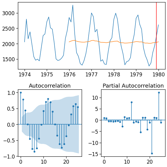
Making forecasts

y_pred = m6.predict(df.index[0], df.index[-1] + pd.Timedelta(1, unit='D') )

fig = plot_ts(y_pred, lags=25)
fig.axes[0].axvline(df.index[-1], c='red')
pass

Bayesian modeling with prophet

! python3 -m pip install --quiet fbprophet

from fbprophet import Prophet

Data needs to have just two columns ds and y.

data = df.reset_index()

m7 = Prophet()

m7 = m7.fit(data)

INFO:fbprophet:Disabling weekly seasonality. Run prophet with weekly_seasonality=True to override this.
INFO:fbprophet:Disabling daily seasonality. Run prophet with daily_seasonality=True to override this.

future = m7.make_future_dataframe(periods=24, freq='M')

forecast = m7.predict(future)

m7.plot(forecast)
pass

Model evaluation

Similarity measures

There are several measures commonly used to evaluate the quality of forecasts. The are the same measures we use to evaluate the fit to any function such as$R^2$, MSE and MAE, so will not be described further here.

Cross-validation

From https://cdn-images-1.medium.com/max/800/1*6ujHlGolRTGvspeUDRe1EA.png

from sklearn.model_selection import TimeSeriesSplit
from sklearn.metrics import mean_squared_error

tsp = TimeSeriesSplit(n_splits=3)

for train, test in tsp.split(df):
    print(train.shape, test.shape)

(18,) (18,)
(36,) (18,)
(54,) (18,)

df.index[train[-1]]

Timestamp('1978-06-01 00:00:00', freq='MS')

df.index[train[-1]+len(test)]

Timestamp('1979-12-01 00:00:00', freq='MS')

A routine like the following can be used for model comparison

res = []
for train, test in tsp.split(df):
    m = Prophet(yearly_seasonality=False, weekly_seasonality=False, daily_seasonality=False)
    m.fit(data.iloc[train])
    future = data[['ds']].iloc[test]
    y_pred = m.predict(future).yhat
    y_true = data.y[test]
    res.append(mean_squared_error(y_true, y_pred))

INFO:fbprophet:n_changepoints greater than number of observations. Using 13.

np.mean(res)

389145.04484811745

If you are using prophet it includees its own diagnostic functions

Prophet is oriented for daily data. At present, it does not appear to support cross-validation for monthly data.