Numbers
The numpy array is the foundation of essentially all numerical computing in Python, so it is important to understand the array and how to use it well.
Learning objectives
Attributes of an array
How to create vectors, matrices, tensors
How to index and slice arrays
Generating random arrays and sampling
Universal functions, vectorization and matrix multiplication
Array axes and marginal calculations
Broadcasting
Masking
Combining and splitting arrays
Vectorizing loops
[1]:
import numpy as np
The ndarray: Vectors, matrices and tenosrs
dtype, shape, strides
Vector
[2]:
x = np.array([1,2,3])
x
[2]:
array([1, 2, 3])
[3]:
type(x)
[3]:
numpy.ndarray
[4]:
x.dtype
[4]:
dtype('int64')
[5]:
x.shape
[5]:
(3,)
[6]:
x.strides
[6]:
(8,)
Matrix
[7]:
x = np.array([[1,2,3], [4,5,6]], dtype=np.int32)
x
[7]:
array([[1, 2, 3],
       [4, 5, 6]], dtype=int32)
[8]:
x.dtype
[8]:
dtype('int32')
[9]:
x.shape
[9]:
(2, 3)
[10]:
x.strides
[10]:
(12, 4)
Tensor
[11]:
x = np.arange(24).reshape((2,3,4))
[12]:
x
[12]:
array([[[ 0,  1,  2,  3],
        [ 4,  5,  6,  7],
        [ 8,  9, 10, 11]],

       [[12, 13, 14, 15],
        [16, 17, 18, 19],
        [20, 21, 22, 23]]])
Creating ndarrays
From a file
[13]:
%%file numbers.txt
a,b,c # can also skip headers
1,2,3
4,5,6
Overwriting numbers.txt
[14]:
np.loadtxt('numbers.txt', dtype='int', delimiter=',',
           skiprows=1, comments='#')
[14]:
array([[1, 2, 3],
       [4, 5, 6]])
From Python lists or tuples
[15]:
np.array([
    [1,2,3],
    [4,5,6]
])
[15]:
array([[1, 2, 3],
       [4, 5, 6]])
From ranges
arange, linspace, logspace
[16]:
np.arange(1, 7).reshape((2,3))
[16]:
array([[1, 2, 3],
       [4, 5, 6]])
[17]:
np.linspace(1, 10, 4)
[17]:
array([ 1., 4., 7., 10.])
[18]:
np.logspace(0, 4, 5, dtype='int')
[18]:
array([ 1, 10, 100, 1000, 10000])
From a function
fromfunciton
[19]:
np.fromfunction(lambda i, j: i*3 + j + 1, (2,3))
[19]:
array([[1., 2., 3.],
       [4., 5., 6.]])
[20]:
np.fromfunction(lambda i, j: (i-2)**2 + (j-2)**2, (5,5), dtype='int')
[20]:
array([[8, 5, 4, 5, 8],
       [5, 2, 1, 2, 5],
       [4, 1, 0, 1, 4],
       [5, 2, 1, 2, 5],
       [8, 5, 4, 5, 8]])
How to visualize fromfunction
[21]:
j = np.repeat([np.arange(5)], 5, axis=0)
i = j.T
[22]:
i
[22]:
array([[0, 0, 0, 0, 0],
       [1, 1, 1, 1, 1],
       [2, 2, 2, 2, 2],
       [3, 3, 3, 3, 3],
       [4, 4, 4, 4, 4]])
[23]:
j
[23]:
array([[0, 1, 2, 3, 4],
       [0, 1, 2, 3, 4],
       [0, 1, 2, 3, 4],
       [0, 1, 2, 3, 4],
       [0, 1, 2, 3, 4]])
[24]:
(i-2)**2 + (j-2)**2
[24]:
array([[8, 5, 4, 5, 8],
       [5, 2, 1, 2, 5],
       [4, 1, 0, 1, 4],
       [5, 2, 1, 2, 5],
       [8, 5, 4, 5, 8]])
Using element-wise functions in fromfunction
[25]:
np.fromfunction(lambda i, j: np.where(i==j,0, -1), (5,5))
[25]:
array([[ 0, -1, -1, -1, -1],
       [-1,  0, -1, -1, -1],
       [-1, -1,  0, -1, -1],
       [-1, -1, -1,  0, -1],
       [-1, -1, -1, -1,  0]])
[26]:
np.fromfunction(lambda i, j: np.where(i<j, 1, np.where(i==j,0, -1)), (5,5))
[26]:
array([[ 0,  1,  1,  1,  1],
       [-1,  0,  1,  1,  1],
       [-1, -1,  0,  1,  1],
       [-1, -1, -1,  0,  1],
       [-1, -1, -1, -1,  0]])
[27]:
np.fromfunction(lambda i, j: np.minimum(i,j), (5,5), dtype='int')
[27]:
array([[0, 0, 0, 0, 0],
       [0, 1, 1, 1, 1],
       [0, 1, 2, 2, 2],
       [0, 1, 2, 3, 3],
       [0, 1, 2, 3, 4]])
[28]:
np.fromfunction(lambda i, j: np.maximum(i,j), (5,5), dtype='int')
[28]:
array([[0, 1, 2, 3, 4],
       [1, 1, 2, 3, 4],
       [2, 2, 2, 3, 4],
       [3, 3, 3, 3, 4],
       [4, 4, 4, 4, 4]])
From special constructors
zeros, ones, eye, diag
[29]:
np.zeros((2,3))
[29]:
array([[0., 0., 0.],
       [0., 0., 0.]])
[30]:
np.ones((2,3))
[30]:
array([[1., 1., 1.],
       [1., 1., 1.]])
[31]:
np.eye(3)
[31]:
array([[1., 0., 0.],
       [0., 1., 0.],
       [0., 0., 1.]])
[32]:
np.eye(3, 4)
[32]:
array([[1., 0., 0., 0.],
       [0., 1., 0., 0.],
       [0., 0., 1., 0.]])
[33]:
np.eye(4, k=-1)
[33]:
array([[0., 0., 0., 0.],
       [1., 0., 0., 0.],
       [0., 1., 0., 0.],
       [0., 0., 1., 0.]])
[34]:
np.diag([1,2,3,4])
[34]:
array([[1, 0, 0, 0],
       [0, 2, 0, 0],
       [0, 0, 3, 0],
       [0, 0, 0, 4]])
[35]:
np.diag([1,2,3,4], k=1)
[35]:
array([[0, 1, 0, 0, 0],
       [0, 0, 2, 0, 0],
       [0, 0, 0, 3, 0],
       [0, 0, 0, 0, 4],
       [0, 0, 0, 0, 0]])
From random variables
Convenience functions
rand, randn
[36]:
np.random.rand(2,3)
[36]:
array([[0.91937873, 0.37638085, 0.18580595],
       [0.2123302 , 0.44596174, 0.60675588]])
[37]:
np.random.randn(2,3)
[37]:
array([[ 0.97230278, -1.46120552, -1.77289026],
       [ 0.44479832, -1.0951637 ,  0.32681921]])
Distributions
uniform, normal, randint, poisson, multinomial, multivariate_ normal
[38]:
np.random.uniform(0, 1, (2,3))
[38]:
array([[0.65654606, 0.47205092, 0.07629729],
       [0.15625553, 0.27920136, 0.88049308]])
[39]:
np.random.normal(0, 1, (2,3))
[39]:
array([[ 1.26753857,  0.6928522 ,  1.16534984],
       [-1.61715447,  0.24027631,  1.29522894]])
[40]:
np.random.randint(0, 10, (4,5))
[40]:
array([[5, 9, 0, 1, 8],
       [4, 0, 9, 6, 7],
       [0, 1, 1, 2, 8],
       [5, 9, 2, 3, 9]])
[41]:
np.random.poisson(10, (4,5))
[41]:
array([[ 4, 12,  6, 10,  8],
       [10, 11,  9,  9, 15],
       [ 8,  7,  7,  6, 10],
       [15,  6,  6,  7,  8]])
[42]:
np.random.multinomial(n=5, pvals=np.ones(5)/5, size=8)
[42]:
array([[0, 4, 0, 1, 0],
       [0, 1, 0, 3, 1],
       [0, 2, 1, 1, 1],
       [1, 1, 1, 0, 2],
       [2, 2, 1, 0, 0],
       [1, 0, 1, 2, 1],
       [0, 1, 1, 2, 1],
       [1, 2, 0, 1, 1]])
[43]:
np.random.multivariate_normal(mean=[10,20,30], cov=np.eye(3), size=4)
[43]:
array([[10.77726641, 18.34924582, 31.54368944],
       [ 9.9150742 , 19.0163889 , 30.5417952 ],
       [ 9.90124065, 20.42154792, 32.69330161],
       [ 8.84846483, 19.53126217, 30.54025679]])
Sampling using choice
Works much like the R sample function.
[44]:
x = np.random.permutation(list('ABCDEF'))
[45]:
x
[45]:
array(['A', 'D', 'F', 'E', 'C', 'B'], dtype='<U1')
[46]:
np.random.choice(x, 3)
[46]:
array(['B', 'E', 'F'], dtype='<U1')
[47]:
np.random.choice(x, 10)
[47]:
array(['A', 'F', 'F', 'D', 'B', 'F', 'D', 'C', 'B', 'A'], dtype='<U1')
[48]:
try:
    np.random.choice(x, 10, replace=False)
except ValueError as e:
    print(e)
Cannot take a larger sample than population when 'replace=False'
Indexing
[49]:
x = np.arange(20).reshape((4,5))
x
[49]:
array([[ 0,  1,  2,  3,  4],
       [ 5,  6,  7,  8,  9],
       [10, 11, 12, 13, 14],
       [15, 16, 17, 18, 19]])
Using slices
[52]:
x[1,:]
[52]:
array([5, 6, 7, 8, 9])
[53]:
x[:,1]
[53]:
array([ 1, 6, 11, 16])
[54]:
x[1:3,1:3]
[54]:
array([[ 6,  7],
       [11, 12]])
Extrcting blocks with arbitrary row and column lists (fancy indexing)
np.ix_
[56]:
x[:, [0,3]]
[56]:
array([[ 0,  3],
       [ 5,  8],
       [10, 13],
       [15, 18]])
Warning: Fancy indexing can only be used for 1 dimension at a time.
In the example below, numpy treats the arguments as paired coordinates, and returns the values at (0,0) and (2,3).
[57]:
x[[0,2],[0,3]]
[57]:
array([ 0, 13])
Use the helper np.ix_ to extract arbitrary blocks.
[58]:
x[np.ix_([0,2], [0,3])]
[58]:
array([[ 0,  3],
       [10, 13]])
A slice is a view, not a copy
Warning
b = a[:]
makes a copy if a is a list but not if a is a numpy array
[59]:
a1 = list(range(3))
a2 = np.arange(3)
[60]:
b = a1[:]
b[1] = 9
a1
[60]:
[0, 1, 2]
[61]:
b = a2[:]
b[1] = 9
a2
[61]:
array([0, 9, 2])
[62]:
x
[62]:
array([[ 0,  1,  2,  3,  4],
       [ 5,  6,  7,  8,  9],
       [10, 11, 12, 13, 14],
       [15, 16, 17, 18, 19]])
[63]:
y = x[1:-1, 1:-1]
y
[63]:
array([[ 6,  7,  8],
       [11, 12, 13]])
[64]:
y *= 10
[65]:
y
[65]:
array([[ 60,  70,  80],
       [110, 120, 130]])
[66]:
x
[66]:
array([[  0,   1,   2,   3,   4],
       [  5,  60,  70,  80,   9],
       [ 10, 110, 120, 130,  14],
       [ 15,  16,  17,  18,  19]])
Use the copy method to convert a view to a copy
[67]:
z = x[1:-1, 1:-1].copy()
[68]:
z
[68]:
array([[ 60,  70,  80],
       [110, 120, 130]])
[69]:
z[:] = 0
[70]:
z
[70]:
array([[0, 0, 0],
       [0, 0, 0]])
[71]:
x
[71]:
array([[  0,   1,   2,   3,   4],
       [  5,  60,  70,  80,   9],
       [ 10, 110, 120, 130,  14],
       [ 15,  16,  17,  18,  19]])
Boolean indexing
[72]:
x[x % 2 == 0]
[72]:
array([ 0, 2, 4, 60, 70, 80, 10, 110, 120, 130, 14, 16, 18])
[73]:
x [x > 3]
[73]:
array([  4,   5,  60,  70,  80,   9,  10, 110, 120, 130,  14,  15,  16,
        17,  18,  19])
Functions that return indexes
[74]:
idx = np.nonzero(x)
idx
[74]:
(array([0, 0, 0, 0, 1, 1, 1, 1, 1, 2, 2, 2, 2, 2, 3, 3, 3, 3, 3]),
 array([1, 2, 3, 4, 0, 1, 2, 3, 4, 0, 1, 2, 3, 4, 0, 1, 2, 3, 4]))
[75]:
x[idx]
[75]:
array([  1,   2,   3,   4,   5,  60,  70,  80,   9,  10, 110, 120, 130,
        14,  15,  16,  17,  18,  19])
[76]:
idx = np.where(x > 3)
idx
[76]:
(array([0, 1, 1, 1, 1, 1, 2, 2, 2, 2, 2, 3, 3, 3, 3, 3]),
 array([4, 0, 1, 2, 3, 4, 0, 1, 2, 3, 4, 0, 1, 2, 3, 4]))
[77]:
x[idx]
[77]:
array([  4,   5,  60,  70,  80,   9,  10, 110, 120, 130,  14,  15,  16,
        17,  18,  19])
Universal functions
[78]:
x
[78]:
array([[  0,   1,   2,   3,   4],
       [  5,  60,  70,  80,   9],
       [ 10, 110, 120, 130,  14],
       [ 15,  16,  17,  18,  19]])
Operations
[79]:
x + x
[79]:
array([[  0,   2,   4,   6,   8],
       [ 10, 120, 140, 160,  18],
       [ 20, 220, 240, 260,  28],
       [ 30,  32,  34,  36,  38]])
Element-wise functions
[80]:
np.log1p(x)
[80]:
array([[0.        , 0.69314718, 1.09861229, 1.38629436, 1.60943791],
       [1.79175947, 4.11087386, 4.26267988, 4.39444915, 2.30258509],
       [2.39789527, 4.7095302 , 4.79579055, 4.87519732, 2.7080502 ],
       [2.77258872, 2.83321334, 2.89037176, 2.94443898, 2.99573227]])
[81]:
x.clip(10, 100)
[81]:
array([[ 10,  10,  10,  10,  10],
       [ 10,  60,  70,  80,  10],
       [ 10, 100, 100, 100,  14],
       [ 15,  16,  17,  18,  19]])
Scans
[82]:
np.cumsum(x, axis=1)
[82]:
array([[  0,   1,   3,   6,  10],
       [  5,  65, 135, 215, 224],
       [ 10, 120, 240, 370, 384],
       [ 15,  31,  48,  66,  85]])
Reductions
[83]:
np.sum(x)
[83]:
703
[84]:
x.prod()
[84]:
0
Margins and the axis argument
[85]:
x
[85]:
array([[  0,   1,   2,   3,   4],
       [  5,  60,  70,  80,   9],
       [ 10, 110, 120, 130,  14],
       [ 15,  16,  17,  18,  19]])
The 0th axis has 4 items, the 1st axis has 5 items.
[86]:
x.shape
[86]:
(4, 5)
[87]:
x.mean()
[87]:
35.15
Marginalizing out the 0th axis = column summaries
[88]:
x.mean(axis=0)
[88]:
array([ 7.5 , 46.75, 52.25, 57.75, 11.5 ])
Marginalizing out the 1st axis = row summaries
[89]:
x.mean(axis=1)
[89]:
array([ 2. , 44.8, 76.8, 17. ])
Note marginalizing out the last axis is a common default.
[90]:
x.mean(axis=-1)
[90]:
array([ 2. , 44.8, 76.8, 17. ])
Marginalization works for higher dimensions in the same way
[91]:
x = np.random.random((2,3,4))
x
[91]:
array([[[0.3336745 , 0.38298878, 0.70668687, 0.56855277],
        [0.90179106, 0.5694977 , 0.62334477, 0.78786623],
        [0.80417192, 0.31019074, 0.61782661, 0.9713464 ]],

       [[0.94828096, 0.96889823, 0.79326191, 0.55329768],
        [0.69623696, 0.57894732, 0.53914262, 0.52367265],
        [0.50338823, 0.58925673, 0.81392667, 0.46841003]]])
[92]:
x.shape
[92]:
(2, 3, 4)
[93]:
x.mean(axis=0).shape
[93]:
(3, 4)
[94]:
x.mean(axis=1).shape
[94]:
(2, 4)
[95]:
x.mean(axis=2).shape
[95]:
(2, 3)
[96]:
x.mean(axis=(0,1)).shape
[96]:
(4,)
[97]:
x.mean(axis=(0,2)).shape
[97]:
(3,)
[98]:
x.mean(axis=(1,2)).shape
[98]:
(2,)
Broadcasting
Broadcasting is what happens when numpy tries to perform binary operations on two arrays with different shapes. In general, shapes are promoted to make the arrays compatible using the following rule
For each axis from highest to lowest
If both dimensions are the same, do nothing
If one of the dimensions is 1 or None and the other is \(k\), promote to \(k\)
Otherwise print error message
[99]:
x = np.zeros((3,2))
x.shape
[99]:
(3, 2)
[100]:
x
[100]:
array([[0., 0.],
       [0., 0.],
       [0., 0.]])
Shapes are compatible
[101]:
y = np.ones(2)
y.shape
[101]:
(2,)
[102]:
x + y
[102]:
array([[1., 1.],
       [1., 1.],
       [1., 1.]])
Shapes are compatible
[103]:
y = np.ones((1,2))
y.shape
[103]:
(1, 2)
[104]:
x + y
[104]:
array([[1., 1.],
       [1., 1.],
       [1., 1.]])
Shapes are incompatible but can be made compaible by adding empty dimension
[105]:
y = np.ones(3)
y.shape
[105]:
(3,)
[106]:
try:
    x + y
except ValueError as e:
    print(e)
operands could not be broadcast together with shapes (3,2) (3,)
[107]:
y[:, None].shape
[107]:
(3, 1)
[108]:
x + y[:, None]
[108]:
array([[1., 1.],
       [1., 1.],
       [1., 1.]])
Shapes are incompatible
[109]:
y = np.ones((2,2))
y.shape
[109]:
(2, 2)
[110]:
try:
    x + y
except ValueError as e:
    print(e)
operands could not be broadcast together with shapes (3,2) (2,2)
More examples of broadcasting
[111]:
x1 = np.arange(12)
[112]:
x1
[112]:
array([ 0, 1, 2, 3, 4, 5, 6, 7, 8, 9, 10, 11])
[113]:
x1 * 10
[113]:
array([ 0, 10, 20, 30, 40, 50, 60, 70, 80, 90, 100, 110])
[114]:
x2 = np.random.randint(0,10,(3,4))
[115]:
x2
[115]:
array([[4, 8, 8, 3],
       [0, 7, 8, 7],
       [1, 4, 8, 7]])
[116]:
x2 * 10
[116]:
array([[40, 80, 80, 30],
       [ 0, 70, 80, 70],
       [10, 40, 80, 70]])
[117]:
x2.shape
[117]:
(3, 4)
Column-wise broadcasting
[118]:
mu = np.mean(x2, axis=0)
mu.shape
[118]:
(4,)
[119]:
x2 - mu
[119]:
array([[ 2.33333333,  1.66666667,  0.        , -2.66666667],
       [-1.66666667,  0.66666667,  0.        ,  1.33333333],
       [-0.66666667, -2.33333333,  0.        ,  1.33333333]])
[120]:
(x2 - mu).mean(axis=0)
[120]:
array([-1.48029737e-16, 2.96059473e-16, 0.00000000e+00, -2.96059473e-16])
Row wise broadcasting
[121]:
mu = np.mean(x2, axis=1)
mu.shape
[121]:
(3,)
[122]:
try:
    x2 - mu
except ValueError as e:
    print(e)
operands could not be broadcast together with shapes (3,4) (3,)
We can add a “dummy” axis using None or np.newaxis
[123]:
mu[:, None].shape
[123]:
(3, 1)
[124]:
x2 - mu[:, None]
[124]:
array([[-1.75,  2.25,  2.25, -2.75],
       [-5.5 ,  1.5 ,  2.5 ,  1.5 ],
       [-4.  , -1.  ,  3.  ,  2.  ]])
[125]:
x2 - mu[:, np.newaxis]
[125]:
array([[-1.75,  2.25,  2.25, -2.75],
       [-5.5 ,  1.5 ,  2.5 ,  1.5 ],
       [-4.  , -1.  ,  3.  ,  2.  ]])
[126]:
np.mean(x2 - mu[:, None], axis=1)
[126]:
array([0., 0., 0.])
Reshaping works too
[127]:
x2 - mu.reshape((-1,1))
[127]:
array([[-1.75,  2.25,  2.25, -2.75],
       [-5.5 ,  1.5 ,  2.5 ,  1.5 ],
       [-4.  , -1.  ,  3.  ,  2.  ]])
Exercise in broadcasting
Creating a 12 by 12 multiplication table
[128]:
x = np.arange(1, 13)
x[:,None] * x[None,:]
[128]:
array([[  1,   2,   3,   4,   5,   6,   7,   8,   9,  10,  11,  12],
       [  2,   4,   6,   8,  10,  12,  14,  16,  18,  20,  22,  24],
       [  3,   6,   9,  12,  15,  18,  21,  24,  27,  30,  33,  36],
       [  4,   8,  12,  16,  20,  24,  28,  32,  36,  40,  44,  48],
       [  5,  10,  15,  20,  25,  30,  35,  40,  45,  50,  55,  60],
       [  6,  12,  18,  24,  30,  36,  42,  48,  54,  60,  66,  72],
       [  7,  14,  21,  28,  35,  42,  49,  56,  63,  70,  77,  84],
       [  8,  16,  24,  32,  40,  48,  56,  64,  72,  80,  88,  96],
       [  9,  18,  27,  36,  45,  54,  63,  72,  81,  90,  99, 108],
       [ 10,  20,  30,  40,  50,  60,  70,  80,  90, 100, 110, 120],
       [ 11,  22,  33,  44,  55,  66,  77,  88,  99, 110, 121, 132],
       [ 12,  24,  36,  48,  60,  72,  84,  96, 108, 120, 132, 144]])
Scaling to have zero mean and unit standard devation for each feature.
[129]:
x = np.random.normal(10, 5,(3,4))
x
[129]:
array([[ 7.56601841,  2.91420426,  9.69736369,  1.24428159],
       [ 5.87862929,  5.98897101, 14.77818785,  8.2864929 ],
       [ 9.6484939 ,  3.2451964 ,  5.10941011,  0.68535071]])
Scaling column-wise
[130]:
(x - x.mean(axis=0))/x.std(axis=0)
[130]:
array([[-0.08541362, -0.82379069, -0.04160329, -0.62477297],
       [-1.17980225,  1.40739857,  1.24501644,  1.41113307],
       [ 1.26521586, -0.58360788, -1.20341315, -0.7863601 ]])
Scaling row-wise
[131]:
(x - x.mean(axis=1)[:, None])/x.std(axis=1)[:, None]
[131]:
array([[ 0.64764447, -0.71523797,  1.27208323, -1.20448974],
       [-0.7884956 , -0.75801539,  1.66987114, -0.12336016],
       [ 1.51979867, -0.43578367,  0.13355165, -1.21756665]])
Masking
[132]:
import numpy.ma as ma
[133]:
x = np.arange(20).reshape(4,5)
[134]:
x
[134]:
array([[ 0,  1,  2,  3,  4],
       [ 5,  6,  7,  8,  9],
       [10, 11, 12, 13, 14],
       [15, 16, 17, 18, 19]])
[135]:
mask = x % 2 == 0
mask
[135]:
array([[ True, False,  True, False,  True],
       [False,  True, False,  True, False],
       [ True, False,  True, False,  True],
       [False,  True, False,  True, False]])
Note that values that are True in the mask are not used in the array
Values that are False are not masked and so remain
So the above mask keeps only the odd numbers in the array
x
[136]:
m = ma.masked_array(x, mask)
[137]:
m
[137]:
masked_array(
  data=[[--, 1, --, 3, --],
        [5, --, 7, --, 9],
        [--, 11, --, 13, --],
        [15, --, 17, --, 19]],
  mask=[[ True, False,  True, False,  True],
        [False,  True, False,  True, False],
        [ True, False,  True, False,  True],
        [False,  True, False,  True, False]],
  fill_value=999999)
[138]:
m.data
[138]:
array([[ 0,  1,  2,  3,  4],
       [ 5,  6,  7,  8,  9],
       [10, 11, 12, 13, 14],
       [15, 16, 17, 18, 19]])
[139]:
m.mask
[139]:
array([[ True, False,  True, False,  True],
       [False,  True, False,  True, False],
       [ True, False,  True, False,  True],
       [False,  True, False,  True, False]])
[140]:
m.sum(axis=0).data
[140]:
array([20, 12, 24, 16, 28])
[141]:
m.sum(axis=1).data
[141]:
array([ 4, 21, 24, 51])
Often used with missing value sentinels
[142]:
import warnings

with warnings.catch_warnings():
    warnings.simplefilter('ignore', RuntimeWarning)
    x1 = x / mask
[143]:
x1
[143]:
array([[ 0., inf,  2., inf,  4.],
       [inf,  6., inf,  8., inf],
       [10., inf, 12., inf, 14.],
       [inf, 16., inf, 18., inf]])
[144]:
x1.sum()
[144]:
inf
[145]:
x2 = ma.masked_invalid(x1)
x2
[145]:
masked_array(
  data=[[0.0, --, 2.0, --, 4.0],
        [--, 6.0, --, 8.0, --],
        [10.0, --, 12.0, --, 14.0],
        [--, 16.0, --, 18.0, --]],
  mask=[[False,  True, False,  True, False],
        [ True, False,  True, False,  True],
        [False,  True, False,  True, False],
        [ True, False,  True, False,  True]],
  fill_value=1e+20)
[146]:
x2.data
[146]:
array([[ 0., inf,  2., inf,  4.],
       [inf,  6., inf,  8., inf],
       [10., inf, 12., inf, 14.],
       [inf, 16., inf, 18., inf]])
[147]:
x2.mask
[147]:
array([[False,  True, False,  True, False],
       [ True, False,  True, False,  True],
       [False,  True, False,  True, False],
       [ True, False,  True, False,  True]])
[148]:
x2.sum()
[148]:
90.0
[149]:
x2.filled(0)
[149]:
array([[ 0.,  0.,  2.,  0.,  4.],
       [ 0.,  6.,  0.,  8.,  0.],
       [10.,  0., 12.,  0., 14.],
       [ 0., 16.,  0., 18.,  0.]])
Combining ndarrays
[150]:
x1 = np.zeros((3,4))
x2 = np.ones((3,5))
x3 = np.eye(4)
[151]:
x1
[151]:
array([[0., 0., 0., 0.],
       [0., 0., 0., 0.],
       [0., 0., 0., 0.]])
[152]:
x2
[152]:
array([[1., 1., 1., 1., 1.],
       [1., 1., 1., 1., 1.],
       [1., 1., 1., 1., 1.]])
[153]:
x3
[153]:
array([[1., 0., 0., 0.],
       [0., 1., 0., 0.],
       [0., 0., 1., 0.],
       [0., 0., 0., 1.]])
Binding rows when number of columns is the same
[154]:
np.r_[x1, x3]
[154]:
array([[0., 0., 0., 0.],
       [0., 0., 0., 0.],
       [0., 0., 0., 0.],
       [1., 0., 0., 0.],
       [0., 1., 0., 0.],
       [0., 0., 1., 0.],
       [0., 0., 0., 1.]])
Binding columns when number of rows is the same
[155]:
np.c_[x1, x2]
[155]:
array([[0., 0., 0., 0., 1., 1., 1., 1., 1.],
       [0., 0., 0., 0., 1., 1., 1., 1., 1.],
       [0., 0., 0., 0., 1., 1., 1., 1., 1.]])
You can combine more than 2 at a time
[156]:
np.c_[x1, x2, x1]
[156]:
array([[0., 0., 0., 0., 1., 1., 1., 1., 1., 0., 0., 0., 0.],
       [0., 0., 0., 0., 1., 1., 1., 1., 1., 0., 0., 0., 0.],
       [0., 0., 0., 0., 1., 1., 1., 1., 1., 0., 0., 0., 0.]])
Stacking
[157]:
np.vstack([x1, x3])
[157]:
array([[0., 0., 0., 0.],
       [0., 0., 0., 0.],
       [0., 0., 0., 0.],
       [1., 0., 0., 0.],
       [0., 1., 0., 0.],
       [0., 0., 1., 0.],
       [0., 0., 0., 1.]])
[158]:
np.hstack([x1, x2])
[158]:
array([[0., 0., 0., 0., 1., 1., 1., 1., 1.],
       [0., 0., 0., 0., 1., 1., 1., 1., 1.],
       [0., 0., 0., 0., 1., 1., 1., 1., 1.]])
[159]:
np.dstack([x2, 2*x2, 3*x2])
[159]:
array([[[1., 2., 3.],
        [1., 2., 3.],
        [1., 2., 3.],
        [1., 2., 3.],
        [1., 2., 3.]],

       [[1., 2., 3.],
        [1., 2., 3.],
        [1., 2., 3.],
        [1., 2., 3.],
        [1., 2., 3.]],

       [[1., 2., 3.],
        [1., 2., 3.],
        [1., 2., 3.],
        [1., 2., 3.],
        [1., 2., 3.]]])
Generic stack with axis argument
[160]:
np.stack([x2, 2*x2, 3*x2], axis=0)
[160]:
array([[[1., 1., 1., 1., 1.],
        [1., 1., 1., 1., 1.],
        [1., 1., 1., 1., 1.]],

       [[2., 2., 2., 2., 2.],
        [2., 2., 2., 2., 2.],
        [2., 2., 2., 2., 2.]],

       [[3., 3., 3., 3., 3.],
        [3., 3., 3., 3., 3.],
        [3., 3., 3., 3., 3.]]])
[161]:
np.stack([x2, 2*x2, 3*x2], axis=1)
[161]:
array([[[1., 1., 1., 1., 1.],
        [2., 2., 2., 2., 2.],
        [3., 3., 3., 3., 3.]],

       [[1., 1., 1., 1., 1.],
        [2., 2., 2., 2., 2.],
        [3., 3., 3., 3., 3.]],

       [[1., 1., 1., 1., 1.],
        [2., 2., 2., 2., 2.],
        [3., 3., 3., 3., 3.]]])
[162]:
np.stack([x2, 2*x2, 3*x2], axis=2)
[162]:
array([[[1., 2., 3.],
        [1., 2., 3.],
        [1., 2., 3.],
        [1., 2., 3.],
        [1., 2., 3.]],

       [[1., 2., 3.],
        [1., 2., 3.],
        [1., 2., 3.],
        [1., 2., 3.],
        [1., 2., 3.]],

       [[1., 2., 3.],
        [1., 2., 3.],
        [1., 2., 3.],
        [1., 2., 3.],
        [1., 2., 3.]]])
Repetition and tiling
For a vector
[163]:
x = np.array([1,2,3])
[164]:
np.repeat(x, 3)
[164]:
array([1, 1, 1, 2, 2, 2, 3, 3, 3])
[165]:
np.tile(x, 3)
[165]:
array([1, 2, 3, 1, 2, 3, 1, 2, 3])
For a matrix
[166]:
x = np.arange(6).reshape((2,3))
x
[166]:
array([[0, 1, 2],
       [3, 4, 5]])
[167]:
np.repeat(x, 3)
[167]:
array([0, 0, 0, 1, 1, 1, 2, 2, 2, 3, 3, 3, 4, 4, 4, 5, 5, 5])
[168]:
np.repeat(x, 3, axis=0)
[168]:
array([[0, 1, 2],
       [0, 1, 2],
       [0, 1, 2],
       [3, 4, 5],
       [3, 4, 5],
       [3, 4, 5]])
[169]:
np.repeat(x, 3, axis=1)
[169]:
array([[0, 0, 0, 1, 1, 1, 2, 2, 2],
       [3, 3, 3, 4, 4, 4, 5, 5, 5]])
[170]:
np.tile(x, (3,2))
[170]:
array([[0, 1, 2, 0, 1, 2],
       [3, 4, 5, 3, 4, 5],
       [0, 1, 2, 0, 1, 2],
       [3, 4, 5, 3, 4, 5],
       [0, 1, 2, 0, 1, 2],
       [3, 4, 5, 3, 4, 5]])
Splitting ndarrays
[171]:
x = np.arange(32).reshape((4,8))
[172]:
x
[172]:
array([[ 0,  1,  2,  3,  4,  5,  6,  7],
       [ 8,  9, 10, 11, 12, 13, 14, 15],
       [16, 17, 18, 19, 20, 21, 22, 23],
       [24, 25, 26, 27, 28, 29, 30, 31]])
[173]:
np.split(x, 4)
[173]:
[array([[0, 1, 2, 3, 4, 5, 6, 7]]),
 array([[ 8,  9, 10, 11, 12, 13, 14, 15]]),
 array([[16, 17, 18, 19, 20, 21, 22, 23]]),
 array([[24, 25, 26, 27, 28, 29, 30, 31]])]
[174]:
np.split(x, 4, axis=1)
[174]:
[array([[ 0,  1],
        [ 8,  9],
        [16, 17],
        [24, 25]]), array([[ 2,  3],
        [10, 11],
        [18, 19],
        [26, 27]]), array([[ 4,  5],
        [12, 13],
        [20, 21],
        [28, 29]]), array([[ 6,  7],
        [14, 15],
        [22, 23],
        [30, 31]])]
Saving and loading arrays
[175]:
x = np.arange(16).reshape(4,4)
y = np.arange(20).reshape(-1,4)
[176]:
np.save('x.npy', x)
[177]:
np.load('x.npy')
[177]:
array([[ 0,  1,  2,  3],
       [ 4,  5,  6,  7],
       [ 8,  9, 10, 11],
       [12, 13, 14, 15]])
[178]:
np.savez('xy.npz', x=x, y=y)
[179]:
arr = np.load('xy.npz')
[180]:
arr['x']
[180]:
array([[ 0,  1,  2,  3],
       [ 4,  5,  6,  7],
       [ 8,  9, 10, 11],
       [12, 13, 14, 15]])
[181]:
arr['y']
[181]:
array([[ 0,  1,  2,  3],
       [ 4,  5,  6,  7],
       [ 8,  9, 10, 11],
       [12, 13, 14, 15],
       [16, 17, 18, 19]])
[182]:
import os
[183]:
os.remove('x.npy')
[184]:
os.remove('xy.npz')
Vectorization
Example 1
The operators and functions (ufuncs) in Python are vectorized, and will work element-wise over all entries in an ndarray.
[185]:
xs = np.zeros(10, dtype='int')
for i in range(10):
    xs[i] = i**2
xs
[185]:
array([ 0, 1, 4, 9, 16, 25, 36, 49, 64, 81])
[186]:
xs = np.arange(10)**2
xs
[186]:
array([ 0, 1, 4, 9, 16, 25, 36, 49, 64, 81])
Using ufuncs
[187]:
np.sqrt(xs)
[187]:
array([0., 1., 2., 3., 4., 5., 6., 7., 8., 9.])
[188]:
np.log1p(xs)
[188]:
array([0.        , 0.69314718, 1.60943791, 2.30258509, 2.83321334,
       3.25809654, 3.61091791, 3.91202301, 4.17438727, 4.40671925])
Example 2
Scalar product.
[189]:
n = 10

xs = np.random.rand(n)
ys = np.random.rand(n)

s = 0
for i in range(n):
    s += xs[i] * ys[i]
s
[189]:
2.147021108520402
[190]:
np.dot(xs, ys)
[190]:
2.147021108520402
[191]:
xs @ ys
[191]:
2.147021108520402
Example 3
[192]:
m = 3
n = 2

alpha = np.random.rand(1)
betas = np.random.rand(n,1)
xs = np.random.rand(m,n)
[193]:
alpha
[193]:
array([0.09337084])
[194]:
betas
[194]:
array([[0.09122522],
       [0.17668402]])
[195]:
xs
[195]:
array([[0.72345868, 0.61856813],
       [0.23926986, 0.07000004],
       [0.40526047, 0.51643171]])
Using loops
[196]:
ys = np.zeros((m,1))
for i in range(m):
    ys[i] = alpha
    for j in range(n):
        ys[i] += betas[j] * xs[i,j]
ys
[196]:
array([[0.26865962],
       [0.12756617],
       [0.22158605]])
Removing inner loop
[197]:
ys = np.zeros((m,1))
for i in range(m):
    ys[i] = alpha + xs[i,:].T @ betas
ys
[197]:
array([[0.26865962],
       [0.12756617],
       [0.22158605]])
Removing all loops
[198]:
ys = alpha + xs @ betas
ys
[198]:
array([[0.26865962],
       [0.12756617],
       [0.22158605]])
Alternative approach
The calculaiton with explicit intercepts and coefficients is common in deep learning, where \(\alpha\) is called the bias (\(b\)) and \(\beta\) are called the weights (\(w\)), and each equation is \(y[i] = b + w[i]*x[i]\).
It is common in statisiics to use an augmented matrix in which the first column is all ones, so that all that is needed is a single matrix multiplicaiotn.
[199]:
X = np.c_[np.ones(m), xs]
X
[199]:
array([[1.        , 0.72345868, 0.61856813],
       [1.        , 0.23926986, 0.07000004],
       [1.        , 0.40526047, 0.51643171]])
[200]:
alpha
[200]:
array([0.09337084])
[201]:
betas
[201]:
array([[0.09122522],
       [0.17668402]])
[202]:
betas_ = np.concatenate([[alpha], betas])
betas_
[202]:
array([[0.09337084],
       [0.09122522],
       [0.17668402]])
[203]:
ys = X @ betas_
ys
[203]:
array([[0.26865962],
       [0.12756617],
       [0.22158605]])
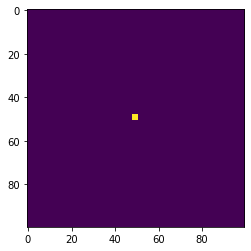
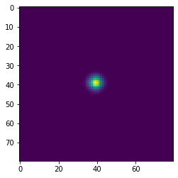
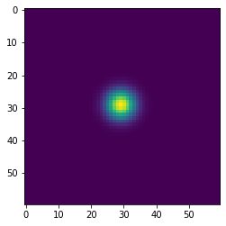
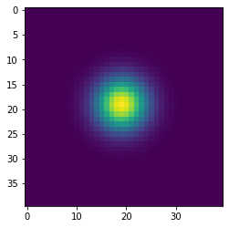
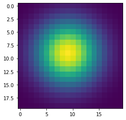
Simulating diffusion
[204]:
%matplotlib inline
import matplotlib.pyplot as plt
[205]:
w = 100
h = 100
x = np.zeros((w+2,h+2), dtype='float')
x[(w//2-1):(w//2+2), (h//2-1):(h//2+2)] = 1

wts = np.ones(5)/5

for i in range(41):
    if i % 10 == 0:
        plt.figure()
        plt.imshow(x[1:-1, 1:-1], interpolation='nearest')

    center = x[1:-1, 1:-1]
    left = x[:-2, 1:-1]
    right = x[2:, 1:-1]
    bottom = x[1:-1, :-2]
    top = x[1:-1, 2:]
    nbrs = np.dstack([center, left, right, bottom, top])
    x = np.sum(wts * nbrs, axis=-1)
[206]: