Constrained Optimization

import numpy as np
from scipy.linalg import cholesky, solve_triangular, cho_solve, cho_factor
from scipy.linalg import solve
from scipy.optimize import minimize

Lagrange multipliers and constrained optimization

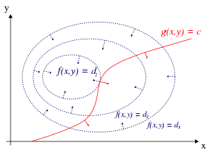
Recall why Lagrange multipliers are useful for constrained optimization - a stationary point must be where the constraint surface \(g\) touches a level set of the function \(f\) (since the value of \(f\) does not change on a level set). At that point, \(f\) and \(g\) are parallel, and hence their gradients are also parallel (since the gradient is normal to the level set). So we want to solve

\[\nabla f = -\lambda \nabla g\]

or equivalently,

\[\nabla f + \lambda \nabla g = 0\]

Example 1

Maximize \(f (x, y, z) = xy + yz\) subject to the constraints \(x + 2y = 6\) and \(x − 3z = 0\).

We set up the equations

\[F (x, y, z, λ, μ) = xy + yz − λ(x + 2y − 6) − μ(x − 3z)\]

Now set partial derivatives to zero and solve the following set of equations

\begin{align} y - \lambda - \mu &= 0 \\ x + z - 2\lambda &= 0 \\ y +3\mu &= 0 \\ x + 2y - 6 &= 0 \\ x - 3z &= 0 \end{align}

which is a linear equation in \(x, y, z, \lambda, \mu\)

\[\begin{split}\begin{pmatrix} 0 & 1 & 0 & -1 & -1 \\ 1 & 0 & 1 & -2 & 0 \\ 0 & 1 & 0 & 0 & 3 \\ 1 & 2 & 0 & 0 & 0 \\ 1 & 0 & -3 & 0 & 0 \\ \end{pmatrix}\pmatrix{x \\ y \\ z \\ \lambda \\ \mu} = \pmatrix{0 \\ 0 \\ 0 \\ 6 \\ 0}\end{split}\]

A = np.array([
    [0, 1, 0, -1, -1],
    [1, 0, 1, -2, 0],
    [0, 1, 0, 0, 3],
    [1, 2, 0, 0, 0],
    [1, 0,-3, 0, 0]])

b = np.array([0,0,0,6,0])

sol = solve(A, b)

sol

array([ 3. ,  1.5,  1. ,  2. , -0.5])

def f(x, y, z):
    return x*y + y*z

f(*sol[:3])

6.0

Using scipy.optimize

We first need to set this as a minimization problem.

def f(x):
    return -(x[0]*x[1] + x[1]*x[2])

cons = ({'type': 'eq',
         'fun' : lambda x: np.array([x[0] + 2*x[1] - 6, x[0] - 3*x[2]])})

x0 = np.array([2,2,0.67])
res = minimize(f, x0, constraints=cons)

res.fun

-5.999999999999969

res.x

array([2.99999979, 1.50000011, 0.99999993])

Example 2

Find the minimum of the following quadratic function on \(\mathbb{R}^2\)

\[ \begin{align}\begin{aligned}f(x) = x^TAx +b^Tx +c\\where\end{aligned}\end{align} \]

\[\begin{split}A = \left(\begin{matrix}13&5\\5&7\end{matrix}\right), b = \left(\begin{matrix}1\\1\end{matrix}\right) \textrm {and } c = 2\end{split}\]

Under the constraints:

\[g(x) = 2x_1-5x_2=2 \;\;\;\;\;\; \textrm{ and } \;\;\;\;\;\; h(x) = x_1+x_2=1\]

1. Use a matrix decomposition method to find the minimum of the unconstrained problem without using scipy.optimize (Use library functions - no need to code your own). Note: for full credit you should exploit matrix structure.

2. Find the solution using constrained optimization with the scipy.optimize package.

3. Use Lagrange multipliers and solving the resulting set of equations directly without using scipy.optimize.

Solve unconstrained problem

To find the minimum, we differentiate \(f(x)\) with respect to \(x^T\) and set it equal to \(0\). We thus need to solve

\[2Ax + b = 0\]

or

\[Ax = -\frac{b}{2}\]

We see that \(A\) is a symmetric positive definite real matrix. Hence we use Cholesky factorization.

Steps

\[\begin{split}L = \text{cholesky}(A) \\ \text{solve } Ly = b \\ \text{solve } L^Tx = y\end{split}\]

A = np.array([
    [13,5],
    [5,7]
])
b = np.array([1,1]).reshape(-1,1)
c = 2

L = cholesky(A, lower=True)
y = solve_triangular(L, -b/2, lower=True)
x = solve_triangular(L.T, y, lower=False)

x

array([[-0.01515152],
       [-0.06060606]])

cho_solve(cho_factor(A), -b/2)

array([[-0.01515152],
       [-0.06060606]])

Solve constrained problem using scipy.optimize

f = lambda x, A, b, c: x.T @ A @ x + b.T @ x + c

from scipy.optimize import minimize

cons = ({'type': 'eq', 'fun': lambda x: 2*x[0] - 5*x[1] - 2},
        {'type': 'eq', 'fun': lambda x: x[0] + x[1] - 1})

res = minimize(f, [0,0], constraints=cons, args=(A, b, c))
res.x

array([1.00000000e+00, 3.41607086e-16])

Solve constrained problem using Lagrange multipliers

We set up the equations

\[F(x_1, x_2, \lambda, \mu) = f + \lambda g + \mu h\]

Sometimes this is written as

\[F(x_1, x_2, \lambda, \mu) = f - \lambda g - \mu h\]

All this means is a final sign change in the estimated values of \(\lambda\) and \(\mu\).

We show the original equations for convenience

\[f(x) = x^TAx +b^Tx +c\]

where

\[\begin{split}A = \left(\begin{matrix}13&5\\5&7\end{matrix}\right), b = \left(\begin{matrix}1\\1\end{matrix}\right) \textrm {and } c = 2\end{split}\]

Under the constraints:

\[g(x) = 2x_1-5x_2=2 \;\;\;\;\;\; \textrm{ and } \;\;\;\;\;\; h(x) = x_1+x_2=1\]

To make the calculations explicit, we rewrite \(F\) as

\[F = 13x_1^2 + 10xy_1x_2+ 7x_2^2 + x_1 + x_2 +2 + \lambda(2x_1 - 5x_2 -2) + \mu(x_1 + x_2 -1)\]

Taking partial derivatives, we get

\[\begin{split}\begin{align} \frac{\delta F}{\delta x_1} &=& 26 x_1 + 10 x_2 + 1 + 2\lambda + \mu &= 0 \\ \frac{\delta F}{\delta x_2} &=& 10 x_1 + 14 x_2 + 1 - 5\lambda + \mu &= 0 \\ \frac{\delta F}{\delta \lambda} &=& 2 x_1 - 5 x_2 -2 &= 0 \\ \frac{\delta F}{\delta \mu} &=& x_1 + x_2 - 1 &= 0 \end{align}\end{split}\]

Plugging in the numbers and expressing in matrix form, we get

\[\begin{split}\begin{bmatrix} 26 & 10 & 2 & 1 \\ 10 & 14 & -5 & 1 \\ 2 & -5 & 0 & 0 \\ 1 & 1 & 0 & 0 \end{bmatrix} \begin{bmatrix} x_1 \\ x_2 \\ \lambda \\ \mu \end{bmatrix} = \begin{bmatrix} -1 \\ -1 \\ 2 \\ 1 \end{bmatrix}\end{split}\]

With a bit of practice, you can probably just write the matrix directly by inspection.

A = np.array([
    [26, 10, 2, 1],
    [10, 14, -5, 1],
    [2, -5, 0, 0],
    [1, 1, 0, 0]
])
b = np.array([-1, -1, 2, 1]).reshape(-1,1)

solve(A, b)

array([[ 1.00000000e+00],
       [-4.37360585e-17],
       [-2.28571429e+00],
       [-2.24285714e+01]])