[1]:
%matplotlib inline
[2]:
import numpy as np
import numpy.random as rng
import matplotlib.pyplot as plt
import seaborn as sns
import pandas as pd
import pymc3 as pm
import scipy.stats as stats
from sklearn.preprocessing import StandardScaler
import daft
WARNING (theano.configdefaults): install mkl with `conda install mkl-service`: No module named 'mkl'
WARNING (theano.tensor.blas): Using NumPy C-API based implementation for BLAS functions.
[3]:
import theano
import theano.tensor as tt
theano.config.warn.round=False
[4]:
import warnings
warnings.simplefilter('ignore', UserWarning)
[5]:
sns.set_context('notebook')
sns.set_style('darkgrid')
Linear regression
We will show how to estimate regression parameters using a simple linear model
We can restate the linear model
as sampling from a probability distribution
Now we can use pymc to estimate the parameters \(a\), \(b\) and \(\sigma\). We will assume the following priors
Note: It may be useful to scale observed values to have zero mean and unit standard deviation to simplify choice of priors. However, you may need to back-transform the parameters to interpret the estimated values.
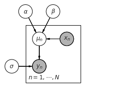
Plate diagram
[6]:
import daft

# Instantiate the PGM.
pgm = daft.PGM(shape=[4.0, 3.0], origin=[-0.3, -0.7])

# Hierarchical parameters.
pgm.add_node(daft.Node("alpha", r"$\alpha$", 0.5, 2))
pgm.add_node(daft.Node("beta", r"$\beta$", 1.5, 2))
pgm.add_node(daft.Node("sigma", r"$\sigma$", 0, 0))

# Deterministic variable.
pgm.add_node(daft.Node("mu", r"$\mu_n$", 1, 1))

# Data.
pgm.add_node(daft.Node("x", r"$x_n$", 2, 1, observed=True))
pgm.add_node(daft.Node("y", r"$y_n$", 1, 0, observed=True))

# Add in the edges.
pgm.add_edge("alpha", "mu")
pgm.add_edge("beta", "mu")
pgm.add_edge("x", "mu")
pgm.add_edge("mu", "y")
pgm.add_edge("sigma", "y")

# And a plate.
pgm.add_plate(daft.Plate([0.5, -0.5, 2, 2], label=r"$n = 1, \cdots, N$",
    shift=-0.1))

# Render and save.
pgm.render()
pgm.figure.savefig("lm.pdf")
Setting up and fitting linear model
[7]:
# observed data
np.random.seed(123)
n = 11
_a = 6
_b = 2
x = np.linspace(0, 1, n)
y = _a*x + _b + np.random.randn(n)
[8]:
niter = 1000
with pm.Model() as linreg:
    a = pm.Normal('a', mu=0, sd=100)
    b = pm.Normal('b', mu=0, sd=100)
    sigma = pm.HalfNormal('sigma', sd=1)

    y_est = a*x + b
    likelihood = pm.Normal('y', mu=y_est, sd=sigma, observed=y)

    trace = pm.sample(niter, random_seed=123)
Auto-assigning NUTS sampler...
Initializing NUTS using jitter+adapt_diag...
Multiprocess sampling (4 chains in 4 jobs)
NUTS: [sigma, b, a]
Sampling 4 chains, 0 divergences: 100%|██████████| 6000/6000 [00:02<00:00, 2309.38draws/s]
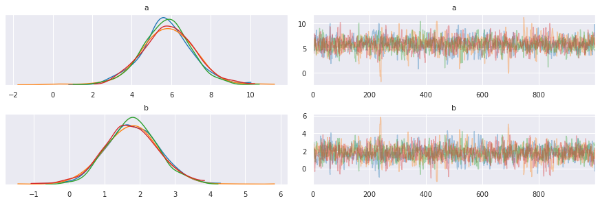
[9]:
pm.traceplot(trace, varnames=['a', 'b'])
pass
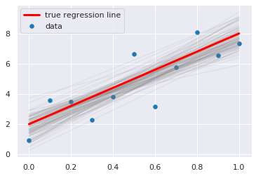
[10]:
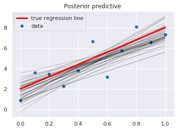
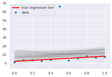
plt.scatter(x, y, s=30, label='data')
for a_, b_ in zip(trace['a'][-100:], trace['b'][-100:]):
    plt.plot(x, a_*x + b_, c='gray', alpha=0.1)
plt.plot(x, _a*x + _b, label='true regression line', lw=3., c='red')
plt.legend(loc='best')
pass
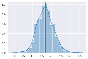
Posterior predictive checks
[11]:
ppc = pm.sample_ppc(trace, samples=500, model=linreg, size=11)
/opt/conda/lib/python3.6/site-packages/ipykernel_launcher.py:1: DeprecationWarning: sample_ppc() is deprecated.  Please use sample_posterior_predictive()
  """Entry point for launching an IPython kernel.
100%|██████████| 500/500 [00:00<00:00, 543.34it/s]
[12]:
sns.distplot([np.mean(n) for n in ppc['y']], kde=True)
plt.axvline(np.mean(y), color='red')
pass
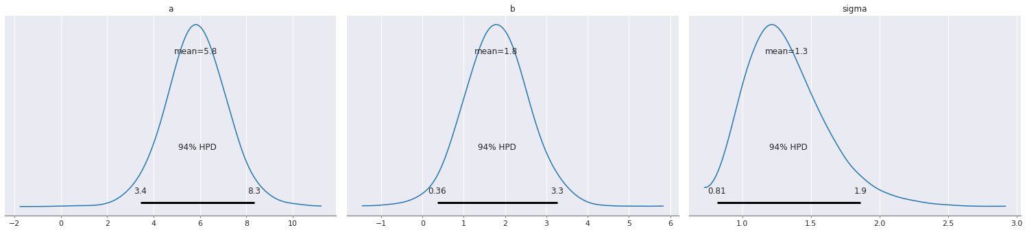
[13]:
pm.plot_posterior(trace)
pass
[14]:
pm.plot_posterior_predictive_glm(
    trace,
    samples=50,
    lm=lambda x, sample: sample['b'] + sample['a'] * x,
)
plt.scatter(x, y, s=30, label='data')
plt.plot(x, _a*x + _b, label='true regression line', lw=3., c='red')
plt.legend(loc='best')
pass
Using the GLM module
Many examples in docs
[15]:
df = pd.DataFrame({'x': x, 'y': y})
df.head()
[15]:
| x | y | |
|---|---|---|
| 0 | 0.0 | 0.914369 |
| 1 | 0.1 | 3.597345 |
| 2 | 0.2 | 3.482978 |
| 3 | 0.3 | 2.293705 |
| 4 | 0.4 | 3.821400 |
[16]:
with pm.Model() as model:
    pm.glm.GLM.from_formula('y ~ x', df)
    trace = pm.sample(2000, tune=1000)
Auto-assigning NUTS sampler...
Initializing NUTS using jitter+adapt_diag...
Multiprocess sampling (4 chains in 4 jobs)
NUTS: [sd, x, Intercept]
Sampling 4 chains, 0 divergences: 100%|██████████| 12000/12000 [00:06<00:00, 1924.53draws/s]
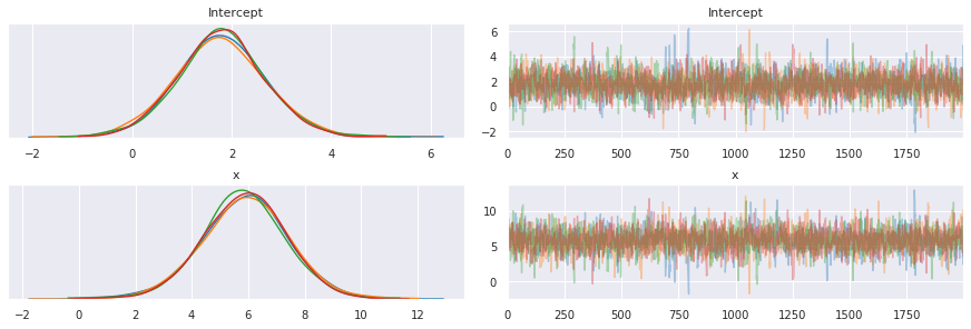
[17]:
pm.traceplot(trace, varnames=['Intercept', 'x'])
pass
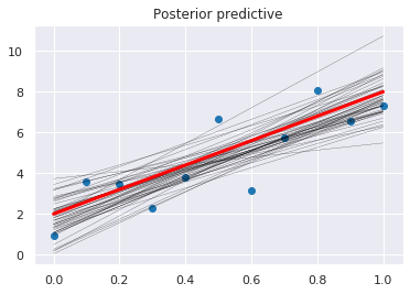
[18]:
plt.scatter(x, y)
pm.plot_posterior_predictive_glm(trace, samples=50)
plt.plot(x, _a*x + _b, label='true regression line', lw=3., c='red')
pass
Robust linear regression
If our data has outliers, we can perform a robust regression by modeling errors from a fatter tailed distribution than the normal distribution.
[19]:
# observed data
np.random.seed(123)
n = 11
_a = 6
_b = 2
x = np.linspace(0, 1, n)
y = _a*x + _b + np.random.randn(n)
y[5] *=10 # create outlier
df = pd.DataFrame({'x': x, 'y': y})
df.head()
[19]:
| x | y | |
|---|---|---|
| 0 | 0.0 | 0.914369 |
| 1 | 0.1 | 3.597345 |
| 2 | 0.2 | 3.482978 |
| 3 | 0.3 | 2.293705 |
| 4 | 0.4 | 3.821400 |
Effect of outlier on linear regression
[20]:
niter = 1000
with pm.Model() as linreg:
    a = pm.Normal('a', mu=0, sd=100)
    b = pm.Normal('b', mu=0, sd=100)
    sigma = pm.HalfNormal('sigma', sd=1)

    y_est = pm.Deterministic('mu', a*x + b)
    y_obs = pm.Normal('y_obs', mu=y_est, sd=sigma, observed=y)

    trace = pm.sample(niter, random_seed=123)
Auto-assigning NUTS sampler...
Initializing NUTS using jitter+adapt_diag...
Multiprocess sampling (4 chains in 4 jobs)
NUTS: [sigma, b, a]
Sampling 4 chains, 0 divergences: 100%|██████████| 6000/6000 [00:03<00:00, 1927.80draws/s]
The acceptance probability does not match the target. It is 0.8829447632025457, but should be close to 0.8. Try to increase the number of tuning steps.
[21]:
with linreg:
    pp = pm.sample_posterior_predictive(trace, samples=100, vars=[a, b])
100%|██████████| 100/100 [00:00<00:00, 9287.45it/s]
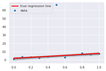
[22]:
plt.scatter(x, y, s=30, label='data')
for a_, b_ in zip(pp['a'], pp['b']):
    plt.plot(x, a_*x + b_, c='gray', alpha=0.1)
plt.plot(x, _a*x + _b, label='true regression line', lw=3., c='red')
plt.legend(loc='upper left')
pass
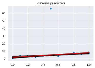
Use a T-distribution for the errors for a more robust fit
Note how we sample [a, b] as a vector β using the shape argument.
[23]:
niter = 1000
with pm.Model() as robust_linreg:
    beta = pm.Normal('beta', 0, 10, shape=2)
    nu = pm.Exponential('nu', 1/len(x))
    sigma = pm.HalfCauchy('sigma', beta=1)

    y_est = beta[0] + beta[1]*x
    y_obs = pm.StudentT('y_obs', mu=y_est, sd=sigma, nu=nu, observed=y)

    trace = pm.sample(niter, random_seed=123)
Auto-assigning NUTS sampler...
Initializing NUTS using jitter+adapt_diag...
Multiprocess sampling (4 chains in 4 jobs)
NUTS: [sigma, nu, beta]
Sampling 4 chains, 0 divergences: 100%|██████████| 6000/6000 [00:04<00:00, 1257.77draws/s]
[24]:
with robust_linreg:
    pp = pm.sample_posterior_predictive(trace, samples=100, vars=[beta])
100%|██████████| 100/100 [00:00<00:00, 10182.08it/s]
[25]:
plt.scatter(x, y, s=30, label='data')
for a_, b_ in zip(pp['beta'][:,1], pp['beta'][:,0]):
    plt.plot(x, a_*x + b_, c='gray', alpha=0.1)
plt.plot(x, _a*x + _b, label='true regression line', lw=3., c='red')
plt.legend(loc='upper left')
pass
Using the GLM module
[26]:
with pm.Model() as model:
    pm.glm.GLM.from_formula('y ~ x', df,
                            family=pm.glm.families.StudentT())
    trace = pm.sample(2000)
Auto-assigning NUTS sampler...
Initializing NUTS using jitter+adapt_diag...
Multiprocess sampling (4 chains in 4 jobs)
NUTS: [lam, x, Intercept]
Sampling 4 chains, 0 divergences: 100%|██████████| 10000/10000 [00:07<00:00, 1389.58draws/s]
[27]:
plt.scatter(x, y)
pm.plot_posterior_predictive_glm(trace, samples=200)
plt.plot(x, _a*x + _b, label='true regression line', lw=3., c='red')
pass
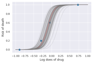
Logistic regression
Gelman’s book has an example where the dose of a drug may be affected to the number of rat deaths in an experiment.
Dose (log g/ml) |
# Rats |
# Deaths |
|---|---|---|
-0.896 |
5 |
0 |
-0.296 |
5 |
1 |
-0.053 |
5 |
3 |
0.727 |
5 |
5 |
We will model the number of deaths as a random sample from a binomial distribution, where \(n\) is the number of rats and \(p\) the probability of a rat dying. We are given \(n = 5\), but we believe that \(p\) may be related to the drug dose \(x\). As \(x\) increases the number of rats dying seems to increase, and since \(p\) is a probability, we use the following model:
where we set vague priors for \(\alpha\) and \(\beta\), the parameters for the logistic model.
Observed data
[28]:
n = 5 * np.ones(4)
x = np.array([-0.896, -0.296, -0.053, 0.727])
y = np.array([0, 1, 3, 5])
[29]:
def invlogit(x):
    return tt.exp(x) / (1 + tt.exp(x))

with pm.Model() as model:
    alpha = pm.Normal('alpha', mu=0, sd=5)
    beta = pm.Flat('beta')

    p = invlogit(alpha + beta*x)
    y_obs = pm.Binomial('y_obs', n=n, p=p, observed=y)

    trace = pm.sample(niter, random_seed=123)
Auto-assigning NUTS sampler...
Initializing NUTS using jitter+adapt_diag...
Multiprocess sampling (4 chains in 4 jobs)
NUTS: [beta, alpha]
Sampling 4 chains, 0 divergences: 100%|██████████| 6000/6000 [00:01<00:00, 3297.61draws/s]
The number of effective samples is smaller than 25% for some parameters.
[30]:
def logit(a, b, xp):
    return np.exp(a + b*xp)/(1 + np.exp(a + b*xp))

with model:
    pp = pm.sample_posterior_predictive(trace, samples=100, vars=[alpha, beta])

xp = np.linspace(-1, 1, 100)
a = trace['alpha'].mean()
b = trace['beta'].mean()
plt.plot(xp, logit(a, b, xp), c='red')

for a_, b_ in zip(pp['alpha'], pp['beta']):
    plt.plot(xp, logit(a_, b, xp), c='gray', alpha=0.2)

plt.scatter(x, y/5, s=50);
plt.xlabel('Log does of drug')
plt.ylabel('Risk of death')
pass
100%|██████████| 100/100 [00:00<00:00, 14660.27it/s]
Hierarchical model
This uses the Gelman radon data set and is based off this IPython notebook. Radon levels were measured in houses from all counties in several states. Here we want to know if the presence of a basement affects the level of radon, and if this is affected by which county the house is located in.

The data set provided is just for the state of Minnesota, which has 85 counties with 2 to 116 measurements per county. We only need 3 columns for this example county, log_radon, floor, where floor=0 indicates that there is a basement.
We will perform simple linear regression on log_radon as a function of county and floor.
[31]:
radon = pd.read_csv('data/radon.csv')[['county', 'floor', 'log_radon']]
radon.head()
[31]:
| county | floor | log_radon | |
|---|---|---|---|
| 0 | AITKIN | 1.0 | 0.832909 |
| 1 | AITKIN | 0.0 | 0.832909 |
| 2 | AITKIN | 0.0 | 1.098612 |
| 3 | AITKIN | 0.0 | 0.095310 |
| 4 | ANOKA | 0.0 | 1.163151 |
In the pooled model, we ignore the county infomraiton.
where \(y\) is the log radon level, and \(x\) an indicator variable for whether there is a basement or not.
We make up some choices for the fairly uniformative priors as usual
However, since the radon level varies by geographical location, it might make sense to include county information in the model. One way to do this is to build a separate regression model for each county, but the sample sizes for some counties may be too small for precise estimates. A compromise between the pooled and separate county models is to use a hierarchical model for patial pooling - the practical efffect of this is to shrink per county estimates towards the group mean, especially for counties with few observations.
Hierarchical model
With a hierarchical model, there is an \(a_c\) and a \(b_c\) for each county \(c\) just as in the individual county model, but they are no longer independent but assumed to come from a common group distribution
we further assume that the hyperparameters come from the following distributions
The variance for observations does not change, so the model for the radon level is
Pooled model
[32]:
niter = 1000
with pm.Model() as pl:
    # County hyperpriors
    mu_a = pm.Normal('mu_a', mu=0, sd=10)
    sigma_a = pm.HalfCauchy('sigma_a', beta=1)
    mu_b = pm.Normal('mu_b', mu=0, sd=10)
    sigma_b = pm.HalfCauchy('sigma_b', beta=1)

    # County slopes and intercepts
    a = pm.Normal('slope', mu=mu_a, sd=sigma_a)
    b = pm.Normal('intercept', mu=mu_b, sd=sigma_b)

    # Houseehold errors
    sigma = pm.Gamma("sigma", alpha=10, beta=1)

    # Model prediction of radon level
    mu = a + b * radon.floor.values

    # Data likelihood
    y = pm.Normal('y', mu=mu, sd=sigma, observed=radon.log_radon)

    pl_trace = pm.sample(niter, tune=5000)
Auto-assigning NUTS sampler...
Initializing NUTS using jitter+adapt_diag...
Multiprocess sampling (4 chains in 4 jobs)
NUTS: [sigma, intercept, slope, sigma_b, mu_b, sigma_a, mu_a]
Sampling 4 chains, 476 divergences: 100%|██████████| 24000/24000 [00:28<00:00, 842.55draws/s]
There were 170 divergences after tuning. Increase `target_accept` or reparameterize.
The acceptance probability does not match the target. It is 0.6245305464723828, but should be close to 0.8. Try to increase the number of tuning steps.
There were 91 divergences after tuning. Increase `target_accept` or reparameterize.
The acceptance probability does not match the target. It is 0.6924175593699173, but should be close to 0.8. Try to increase the number of tuning steps.
There were 89 divergences after tuning. Increase `target_accept` or reparameterize.
The acceptance probability does not match the target. It is 0.6465975998152032, but should be close to 0.8. Try to increase the number of tuning steps.
There were 126 divergences after tuning. Increase `target_accept` or reparameterize.
The acceptance probability does not match the target. It is 0.6284491853810067, but should be close to 0.8. Try to increase the number of tuning steps.
The estimated number of effective samples is smaller than 200 for some parameters.
[33]:
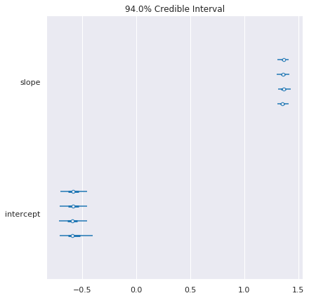
pm.forestplot(pl_trace, varnames=['slope', 'intercept'])
pass
Hierarchical model
[34]:
county = pd.Categorical(radon['county']).codes

niter = 1000
with pm.Model() as hm:
    # County hyperpriors
    mu_a = pm.Normal('mu_a', mu=0, sd=10)
    sigma_a = pm.HalfCauchy('sigma_a', beta=1)
    mu_b = pm.Normal('mu_b', mu=0, sd=10)
    sigma_b = pm.HalfCauchy('sigma_b', beta=1)

    # County slopes and intercepts
    a = pm.Normal('slope', mu=mu_a, sd=sigma_a, shape=len(set(county)))
    b = pm.Normal('intercept', mu=mu_b, sd=sigma_b, shape=len(set(county)))

    # Houseehold errors
    sigma = pm.Gamma("sigma", alpha=10, beta=1)

    # Model prediction of radon level
    mu = a[county] + b[county] * radon.floor.values

    # Data likelihood
    y = pm.Normal('y', mu=mu, sd=sigma, observed=radon.log_radon)

    hm_trace = pm.sample(niter, tune=5000)
Auto-assigning NUTS sampler...
Initializing NUTS using jitter+adapt_diag...
Multiprocess sampling (4 chains in 4 jobs)
NUTS: [sigma, intercept, slope, sigma_b, mu_b, sigma_a, mu_a]
Sampling 4 chains, 142 divergences: 100%|██████████| 24000/24000 [00:43<00:00, 545.52draws/s]
There were 5 divergences after tuning. Increase `target_accept` or reparameterize.
There were 14 divergences after tuning. Increase `target_accept` or reparameterize.
The acceptance probability does not match the target. It is 0.600835238837059, but should be close to 0.8. Try to increase the number of tuning steps.
There were 59 divergences after tuning. Increase `target_accept` or reparameterize.
The acceptance probability does not match the target. It is 0.6605318648750905, but should be close to 0.8. Try to increase the number of tuning steps.
There were 64 divergences after tuning. Increase `target_accept` or reparameterize.
The acceptance probability does not match the target. It is 0.6260419139182648, but should be close to 0.8. Try to increase the number of tuning steps.
The rhat statistic is larger than 1.05 for some parameters. This indicates slight problems during sampling.
The estimated number of effective samples is smaller than 200 for some parameters.
Compare the length of the credible interval with the number of observations for each county.
[35]:
cat = pd.Categorical(radon['county'])
pd.DataFrame(dict(
    code=range(len(cat.categories)),
    n=pd.value_counts(pd.Categorical(radon['county']), sort=False),
)).sort_values('n')
[35]:
| code | n | |
|---|---|---|
| WILKIN | 81 | 1 |
| MAHNOMEN | 41 | 1 |
| MURRAY | 49 | 1 |
| YELLOW MEDICINE | 84 | 2 |
| LAC QUI PARLE | 35 | 2 |
| ... | ... | ... |
| WASHINGTON | 79 | 46 |
| ANOKA | 1 | 52 |
| DAKOTA | 18 | 63 |
| HENNEPIN | 25 | 105 |
| ST LOUIS | 69 | 116 |
85 rows × 2 columns
[36]:
pm.forestplot(hm_trace, varnames=['slope', 'intercept'])
pass

Comparing models
[37]:
df_loo = pm.compare({'pooled': pl_trace, 'hierarchical': hm_trace}, ic='LOO')
df_loo
[37]:
| rank | loo | p_loo | d_loo | weight | se | dse | warning | loo_scale | |
|---|---|---|---|---|---|---|---|---|---|
| hierarchical | 0 | 2077.45 | 64.7044 | 0 | 0.999998 | 51.2026 | 0 | True | deviance |
| pooled | 1 | 2180.07 | 3.84498 | 102.615 | 2.29798e-06 | 58.0256 | 22.9131 | False | deviance |
[38]:
df_waic = pm.compare({'pooled': pl_trace, 'hierarchical': hm_trace}, ic='WAIC')
df_waic
[38]:
| rank | waic | p_waic | d_waic | weight | se | dse | warning | waic_scale | |
|---|---|---|---|---|---|---|---|---|---|
| hierarchical | 0 | 2074.97 | 63.4663 | 0 | 1 | 49.9066 | 0 | True | deviance |
| pooled | 1 | 2180.07 | 3.84783 | 105.097 | 5.08124e-09 | 57.3497 | 22.7185 | False | deviance |
[ ]: