Using ipyparallel

Parallel execution is tightly integrated with Jupyter in the ipyparallel package. Install with

pip install ipyparallel

This is a rich framework. For more on how to use ipyparallel, see

Official documentation

%matplotlib inline
import numpy as np
import matplotlib.pyplot as plt

Starting engines

We will only use engines on local cores which does not require any setup - see docs for detailed instructions on how to set up a remote cluster, including setting up to use Amazon EC2 clusters.

You can start a cluster on the IPython Clusters tab in the main Jupyter browser window

The main advantage of developing parallel applications using ipyparallel is that it can be done interactively within Jupyter.

Basic concepts of ipyparallel

from ipyparallel import Client

The client connects to the cluster of “remote” engines that perfrom the actual computation. These engines may be on the same machine or on a cluster.

rc = Client()

rc.ids

[0, 1, 2, 3, 4, 5, 6, 7]

A view provides access to a subset of the engines available to the client. Jobs are submitted to the engines via the view. A direct view allows the user to explicitly send work specific engines. The load balanced view is like the Pool object in multiprocessing, and manages the scheduling and distribution of jobs for you.

Direct view

dv = rc[:]

Add 10 sets of 3 numbers in parallel using all engines.

dv.map_sync(lambda x, y, z: x + y + z, range(10), range(10), range(10))

[0, 3, 6, 9, 12, 15, 18, 21, 24, 27]

Add 10 sets of 3 numbers in parallel using only alternate engines.

rc[::2].map_sync(lambda x, y, z: x + y + z, range(10), range(10), range(10))

[0, 3, 6, 9, 12, 15, 18, 21, 24, 27]

Add 10 sets of 3 numbers using a specific engine.

rc[2].map_sync(lambda x, y, z: x + y + z, range(10), range(10), range(10))

[0, 3, 6, 9, 12, 15, 18, 21, 24, 27]

Load balanced view

Use this when you have many jobs that take different amounts of time to complete.

lv = rc.load_balanced_view()

lv.map_sync(lambda x: sum(x), np.random.random((10, 100000)))

[49981.15094681111,
 49960.0120441638,
 49890.77961950656,
 49918.427545315106,
 50009.64737591964,
 49959.012023061194,
 50060.41833565818,
 49891.862160926394,
 49932.78181816447,
 50113.55074503267]

Calling functions with apply

In contrast to map, apply is just a simple function call run on all remote engines, and has the usual function signature apply(f, *args, **kwargs). It is a primitive on which other more useful functions (such as map) are built upon.

rc[1:3].apply_sync(lambda x, y: x**2 + y**2, 3, 4)

[25, 25]

rc[1:3].apply_sync(lambda x, y: x**2 + y**2, x=3, y=4)

[25, 25]

Synchronous and asynchronous jobs

We have used the map_sync and apply_sync methods. The sync suffix indicate that we want to run a synchronous job. Synchronous jobs block until all the computation is done and return the result.

res = dv.map_sync(lambda x, y, z: x + y + z, range(10), range(10), range(10))

res

[0, 3, 6, 9, 12, 15, 18, 21, 24, 27]

In contrast, asynchronous jobs return immediately so that you can do other work, but returns a AsyncMapResult object, similar to the future object returned by the concurrent.futures package. You can query its status, cancel running jobs and retrieve results once they have been computed.

res = dv.map_async(lambda x, y, z: x + y + z, range(10), range(10), range(10))

res

<AsyncMapResult: <lambda>>

res.done()

True

res.get()

[0, 3, 6, 9, 12, 15, 18, 21, 24, 27]

There is also a map method that by default uses asynchronous mode, but you can change this by setting the block attribute or function argument.

res = dv.map(lambda x, y, z: x + y + z, range(10), range(10), range(10))

res.get()

[0, 3, 6, 9, 12, 15, 18, 21, 24, 27]

Change blocking mode for just one job.

res = dv.map(lambda x, y, z: x + y + z, range(10), range(10), range(10), block=True)

res

[0, 3, 6, 9, 12, 15, 18, 21, 24, 27]

Change blocking mode for this view so that all jobs are synchronous.

dv.block = True

res = dv.map(lambda x, y, z: x + y + z, range(10), range(10), range(10))

res

[0, 3, 6, 9, 12, 15, 18, 21, 24, 27]

Remote function decorators

The @remote decorator results in functions that will execute simultaneously on all engines in a view. For example, you can use this decorator if you always want to run \(n\) independent parallel MCMC chains.

with dv.sync_imports():
    import numpy

importing numpy on engine(s)

@dv.remote(block = True)
def f1(n):
    return numpy.random.rand(n)

f1(4)

[array([0.18472276, 0.58311062, 0.00970686, 0.82963292]),
 array([0.3707495 , 0.55731368, 0.28422286, 0.11945056]),
 array([0.76889473, 0.16928617, 0.87105353, 0.69520204]),
 array([0.77968322, 0.09836705, 0.29899082, 0.43869955]),
 array([0.44118982, 0.22560375, 0.79489356, 0.78417991]),
 array([0.40955816, 0.31819581, 0.45670871, 0.54122942]),
 array([0.55517265, 0.52965973, 0.12639326, 0.61261257]),
 array([0.07980547, 0.47902453, 0.42447179, 0.41533817])]

The @parallel decorator breaks up elementwise operations and distributes them.

@dv.parallel(block = True)
def f2(x):
    return x

f2(range(15))

[range(0, 2),
 range(2, 4),
 range(4, 6),
 range(6, 8),
 range(8, 10),
 range(10, 12),
 range(12, 14),
 range(14, 15)]

@dv.parallel(block = True)
def f3(x):
    return sum(x)

f3(range(15))

[1, 5, 9, 13, 17, 21, 25, 14]

@dv.parallel(block = True)
def f4(x, y):
    return x + y

f4(np.arange(10), np.arange(10))

array([ 0,  2,  4,  6,  8, 10, 12, 14, 16, 18])

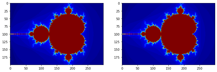
Example: Use the @parallel decorator to speed up Mandelbrot calculations

def mandel1(x, y, max_iters=80):
    c = complex(x, y)
    z = 0.0j
    for i in range(max_iters):
        z = z*z + c
        if z.real*z.real + z.imag*z.imag >= 4:
            return i
    return max_iters

@dv.parallel(block = True)
def mandel2(x, y, max_iters=80):
    c = complex(x, y)
    z = 0.0j
    for i in range(max_iters):
        z = z*z + c
        if z.real*z.real + z.imag*z.imag >= 4:
            return i
    return max_iters

x = np.arange(-2, 1, 0.01)
y = np.arange(-1, 1, 0.01)
X, Y = np.meshgrid(x, y)

%%time
im1 = np.reshape(list(map(mandel1, X.ravel(), Y.ravel())), (len(y), len(x)))

CPU times: user 500 ms, sys: 0 ns, total: 500 ms
Wall time: 500 ms

%%time
im2 = np.reshape(mandel2.map(X.ravel(), Y.ravel()),  (len(y), len(x)))

CPU times: user 32 ms, sys: 8 ms, total: 40 ms
Wall time: 142 ms

fig, axes = plt.subplots(1, 2, figsize=(12, 4))
axes[0].grid(False)
axes[0].imshow(im1, cmap='jet')
axes[1].grid(False)
axes[1].imshow(im2, cmap='jet')
pass

Functions with dependencies

Modules imported locally are NOT available in the remote engines.

import time
import datetime

def g1(x):
    time.sleep(0.1)
    now = datetime.datetime.now()
    return (now, x)

This fails with an Exception because the time and datetime modules are not imported in the remote engines.

dv.map_sync(g1, range(10))

The simplest fix is to import the module(s) within the function

def g2(x):
    import time, datetime
    time.sleep(0.1)
    now = datetime.datetime.now()
    return (now, x)

dv.map_sync(g2, range(5))

[(datetime.datetime(2020, 4, 16, 18, 59, 0, 905717), 0),
 (datetime.datetime(2020, 4, 16, 18, 59, 0, 905823), 1),
 (datetime.datetime(2020, 4, 16, 18, 59, 0, 905938), 2),
 (datetime.datetime(2020, 4, 16, 18, 59, 0, 905981), 3),
 (datetime.datetime(2020, 4, 16, 18, 59, 0, 905971), 4)]

Alternatively, you can simultaneously import both locally and in the remote engines with the sync_import context manager.

with dv.sync_imports():
    import time
    import datetime

importing time on engine(s)
importing datetime on engine(s)

Now the g1 function will work.

dv.map_sync(g1, range(5))

[(datetime.datetime(2020, 4, 16, 18, 59, 1, 76582), 0),
 (datetime.datetime(2020, 4, 16, 18, 59, 1, 76747), 1),
 (datetime.datetime(2020, 4, 16, 18, 59, 1, 76795), 2),
 (datetime.datetime(2020, 4, 16, 18, 59, 1, 77072), 3),
 (datetime.datetime(2020, 4, 16, 18, 59, 1, 77054), 4)]

Finally, there is also a require decorator that can be used. This will force the remote engine to import all packages given.

from ipyparallel import require

@require('scipy.stats')
def g3(x):
    return scipy.stats.norm(0,1).pdf(x)

dv.map(g3, np.arange(-3, 4))

[0.0044318484119380075,
 0.05399096651318806,
 0.24197072451914337,
 0.3989422804014327,
 0.24197072451914337,
 0.05399096651318806,
 0.0044318484119380075]

Moving data around

We can send data to remote engines with push and retrieve them with pull, or using the dictionary interface. For example, you can use this to distribute a large lookup table to all engines once instead of repeatedly as a function argument.

dv.push(dict(a=3, b=2))

[None, None, None, None, None, None, None, None]

def f(x):
    global a, b
    return a*x + b

dv.map_sync(f, range(5))

[2, 5, 8, 11, 14]

dv.pull(('a', 'b'))

[[3, 2], [3, 2], [3, 2], [3, 2], [3, 2], [3, 2], [3, 2], [3, 2]]

You can also use the dictionary interface as an alternative to push and pull

dv['c'] = 5

dv['a']

[3, 3, 3, 3, 3, 3, 3, 3]

dv['c']

[5, 5, 5, 5, 5, 5, 5, 5]

Using parallel magic commands

In practice, most users will simply use the %px magic to execute code in parallel from within the notebook. This is the simplest way to use ipyparallel.

def f(xs):
    s = 0
    for x in xs:
        s += x
    return s

dv.map(f, np.random.random((6, 4)))

[1.455821873914668,
 2.5548527878771496,
 1.943134943296887,
 3.5219170200603296,
 3.5108098284842204,
 1.8450153390831912]

This sends the command to all targeted engines.

%px import numpy as np
%px a = np.random.random(4)
%px a.sum()

Out[0:3]: 1.231755492630267

Out[1:3]: 2.6964804654703194

Out[2:3]: 2.7872819711433436

Out[3:3]: 2.2651690765222607

Out[4:3]: 2.538202038021672

Out[5:3]: 2.342684993836116

Out[6:3]: 1.2899226452213557

Out[7:3]: 1.402290461197728

List comprehensions in parallel

The scatter method partitions and distributes data to all engines. The gather method does the reverse. Together with %px, we can simulate parallel list comprehensions.

dv.scatter('a', np.random.randint(0, 10, 10))
%px print(a)

[stdout:0] [9 7]
[stdout:1] [0 9]
[stdout:2] [3]
[stdout:3] [2]
[stdout:4] [9]
[stdout:5] [9]
[stdout:6] [8]
[stdout:7] [5]

dv.gather('a')

array([9, 7, 0, 9, 3, 2, 9, 9, 8, 5])

dv.scatter('xs', range(24))
%px y = [x**2 for x in xs]
np.array(dv.gather('y'))

array([  0,   1,   4,   9,  16,  25,  36,  49,  64,  81, 100, 121, 144,
       169, 196, 225, 256, 289, 324, 361, 400, 441, 484, 529])

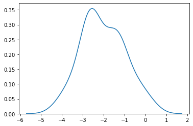
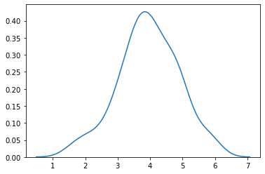
Running magic functions in parallel

%%px --target [1,3]
%matplotlib inline
import seaborn as sns
x = np.random.normal(np.random.randint(-10, 10), 1, 100)
sns.kdeplot(x);

[output:1]

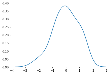
[output:3]

Running in non-blocking mode

%%px --target [1,3] --noblock
%matplotlib inline
import seaborn as sns
x = np.random.normal(np.random.randint(-10, 10), 1, 100)
sns.kdeplot(x);

<AsyncResult: execute>

%pxresult

[output:1]

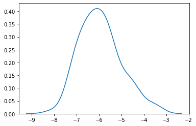
[output:3]