Vectors

Informally, we think of a vector as an object that has magnitude and direction. More formally, we think of an \(n\)-dimensional vector as an ordered tuple of numbers \((x_1, x_2, \ldots, x_n)\) that follows the rules of scalar multiplication and vector addition.

%matplotlib inline

import numpy as np
import matplotlib.pyplot as plt

Vector space

A vector space is a collection of vectors which is closed under addition and scalar multiplication.

Examples:

• Euclidean plane \(\mathbb{R}^2\) is a familiar vector space

• The vector \(\pmatrix{0 & 0}\) is a trivial vector space that is a vector subspace of Euclidean space.

• Polynomial functions of order \(k\) is a vector space

Polynomials of order 3 have the form \(ax^3 + bx^2 + cx + d\), and can be represented as the vector

\[\begin{split}\pmatrix{a \\ b \\ c \\ d}\end{split}\]

• The space of all continuous functions is a vector space

Consider two continuous functions, say, \(f(x) = x^2\) and \(g(x) = x^3)\). Scalar multiplication \((2 f)(x) = 2x^2\) and addition \((f + g)(x) = x^2 + x^3\) are well defined and the result is a continuous function, so the space of all continuous functions is also a vector space. In this case, it is an infinite-dimensional vector space.

Vector spaces are important because the theorems of linear algebra apply to all vector spaces, not just Euclidean space.

Column vectors

When we describe a vector \(x\), we mean the column vector. The row vector is denoted \(x^T\).

x = np.random.random((5,1))
x

array([[0.61203208],
       [0.98286311],
       [0.98038756],
       [0.81615497],
       [0.75487332]])

x.T

array([[0.61203208, 0.98286311, 0.98038756, 0.81615497, 0.75487332]])

Dimensions

len(x)

5

Length

The length of a vector is the Euclidean norm (i.e. Pythagoras theorem)

np.linalg.norm(x)

1.8808789368516818

np.sqrt(np.sum(x**2))

1.8808789368516818

Direction

n = x/np.linalg.norm(x)
n

array([[0.32539685],
       [0.52255522],
       [0.52123905],
       [0.43392212],
       [0.40134073]])

np.linalg.norm(n)

1.0

Norms and distances

Recall that the ‘norm’ of a vector \(v\), denoted \(||v||\) is simply its length. For a vector with components

\[ \begin{align}\begin{aligned}v = \left(v_1,...,v_n\right)\\the norm of :math:`v` is given by:\end{aligned}\end{align} \]

\[||v|| = \sqrt{v_1^2+...+v_n^2}\]

The distance between two vectors is the length of their difference:

\[d(v,w) = ||v-w||\]

u = np.array([3,0]).reshape((-1,1))
v = np.array([0,4]).reshape((-1,1))

np.linalg.norm(u - v)

5.0

np.linalg.norm(v - u)

5.0

np.sqrt(np.sum((u - v)**2))

5.0

Vector operations

x = np.arange(3).reshape((-1,1))
y = np.arange(3).reshape((-1,1))

3 * x

array([[0],
       [3],
       [6]])

x + y

array([[0],
       [2],
       [4]])

3*x + 4*y

array([[ 0],
       [ 7],
       [14]])

x.T

array([[0, 1, 2]])

Dot product

The dot product of two vectors \(u\) and \(v\) is written as \(u \cdot v\) and its value is given by \(u^Tv\). The dot product of two \(n\) dimensional vectors \(v\) and \(w\) is given by:

\[u \cdot v = u_1v_1+...+u_nv_n\]

I.e. the dot product is just the sum of the product of the components.

The inner product \(\langle u,v \rangle\) of two vectors is a generalization of the dot product. It is any function that takes two vectors, returns a scalar (here we just consider inner products that return real numbers), and obeys the following properties:

• symmetry \(\langle u,v \rangle = \langle v,u \rangle\)

• positive definite

  • \(\langle v,v \rangle \ge 0\)

  • \(\langle v,v \rangle = 0 \implies v = 0\)

• bilinear

  • \(\langle au,v \rangle = a \langle u,v \rangle\)

  • \(\langle u + v,w \rangle = \langle u,w \rangle + \langle v,w \rangle\)

  • Linearity also applies to second argument because of symmetry

Any inner product determines a norm via:

\[||v|| = \langle v,v \rangle^{\frac12}\]

u = np.array([3,3]).reshape((-1,1))
v = np.array([2,0]).reshape((-1,1))

np.dot(u.T, v)

array([[6]])

You can also use the @ operator to do matrix multiplication

u.T @ v

array([[6]])

np.sum(u * v)

6

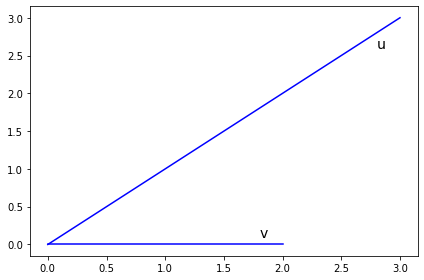
Geometrically, the dot product is the product of the length of \(v\) and the length of the projection of \(u\) onto the unit vector \(\widehat{v}\).

\[u \cdot v = \lvert u \rvert \lvert v \rvert \cos \theta\]

plt.plot(*zip(np.zeros_like(u), u), 'b-')
plt.text(1.8, 0.1, 'v', fontsize=14)
plt.plot(*zip(np.zeros_like(v), v), 'b-')
plt.text(2.8, 2.6, 'u', fontsize=14)
plt.tight_layout()
pass

cos_angle = np.dot(u.T, v)/(np.linalg.norm(u)*np.linalg.norm(v))

cos_angle

array([[0.70710678]])

theta = 180/np.pi*np.arccos(cos_angle)

theta

array([[45.]])

Outer product

Note that the inner product is just matrix multiplication of a \(1\times n\) vector with an \(n\times 1\) vector. In fact, we may write:

\[\langle v,w \rangle = v^Tw\]

The outer product of two vectors is just the opposite. It is given by:

\[v\otimes w = vw^T\]

Note that I am considering \(v\) and \(w\) as column vectors. The result of the inner product is a scalar. The result of the outer product is a matrix.

For example, if \(v\) and \(w\) are both in \(\mathbb{R}^3\)

\[\begin{split}v \otimes w = \pmatrix{v_1\\v_2\\v_3} \pmatrix{w_1 & w_2 & w_3} = \pmatrix{ v_1w_1 & v_1w_2 & v_1w_3\\ v_2w_1 & v_2w_2 & v_2w_3 \\ v_3w_1 & v_3w_2 & v_3w_3}\end{split}\]

v = np.array([1,2,3]).reshape((-1,1))

v

array([[1],
       [2],
       [3]])

v @ v.T

array([[1, 2, 3],
       [2, 4, 6],
       [3, 6, 9]])

np.outer(v, v)

array([[1, 2, 3],
       [2, 4, 6],
       [3, 6, 9]])