[1]:
%matplotlib inline

import matplotlib.pyplot as plt
import numpy as np
from scipy import stats
Monte Carlo integration
Integrals and averates
In general, we want to estimate integrals of a function over a distribution using the following simple strategy:
Draw a probability from the target probability distribution
Multiply the probability with the function at that value
Repeat and average
The trick is in knowing how to draw samples from the target probability distribution.
A Simple Method: Rejection sampling
Suppose we want random samples from some distribution for which we can calculate the PDF at a point, but lack a direct way to generate random deviates from. One simple idea that is also used in MCMC is rejection sampling - first generate a sample from a distribution from which we can draw samples (e.g. uniform or normal), and then accept or reject this sample with some probability (see figure).
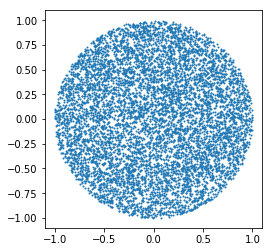
Example: Random samples from the unit circle using rejection sampling
[2]:
x = np.random.uniform(-1, 1, (10000, 2))
x = x[np.sum(x**2, axis=1) < 1]
plt.scatter(x[:, 0], x[:,1], s=1)
plt.axis('square')
pass
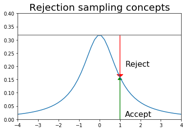
Example: Rejection sampling from uniform distribution
We want to draw samples from a Cauchy distribution restricted to (-4, 4). We could choose a more efficient sampling/proposal distribution than the uniform, but this is just to illustrate the concept.
[3]:
x = np.linspace(-4, 4)

df = 10
dist = stats.cauchy()
upper = dist.pdf(0)
[4]:
plt.plot(x, dist.pdf(x))
plt.axhline(upper, color='grey')
px = 1.0
plt.arrow(px,0,0,dist.pdf(1.0)-0.01, linewidth=1,
          head_width=0.2, head_length=0.01, fc='g', ec='g')
plt.arrow(px,upper,0,-(upper-dist.pdf(px)-0.01), linewidth=1,
          head_width=0.3, head_length=0.01, fc='r', ec='r')
plt.text(px+.25, 0.2, 'Reject', fontsize=16)
plt.text(px+.25, 0.01, 'Accept', fontsize=16)
plt.axis([-4,4,0,0.4])
plt.title('Rejection sampling concepts', fontsize=20)
pass
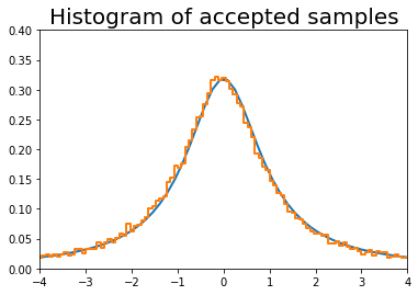
[5]:
n = 100000
# generate from sampling distribution
u = np.random.uniform(-4, 4, n)
# accept-reject criterion for each point in sampling distribution
r = np.random.uniform(0, upper, n)
# accepted points will come from target (Cauchy) distribution
v = u[r < dist.pdf(u)]

plt.plot(x, dist.pdf(x), linewidth=2)

# Plot scaled histogram
factor = dist.cdf(4) - dist.cdf(-4)
hist, bin_edges = np.histogram(v, bins=100, normed=True)
bin_centers = (bin_edges[:-1] + bin_edges[1:]) / 2.
plt.step(bin_centers, factor*hist, linewidth=2)

plt.axis([-4,4,0,0.4])
plt.title('Histogram of accepted samples', fontsize=20)
pass
/Users/cliburn/Library/Python/3.7/lib/python/site-packages/ipykernel_launcher.py:13: VisibleDeprecationWarning: Passing `normed=True` on non-uniform bins has always been broken, and computes neither the probability density function nor the probability mass function. The result is only correct if the bins are uniform, when density=True will produce the same result anyway. The argument will be removed in a future version of numpy.
  del sys.path[0]
Simple Monte Carlo integration
The basic idea of Monte Carlo integration is very simple and only requires elementary statistics. Suppose we want to find the value of
In a statistical context, we use Monte Carlo integration to estimate the expectation
with
We can estimate the Monte Carlo variance of the approximation as
Also, from the Central Limit Theorem,
The convergence of Monte Carlo integration is \(\mathcal{0}(n^{1/2})\) and independent of the dimensionality. Hence Monte Carlo integration generally beats numerical integration for moderate- and high-dimensional integration since numerical integration (quadrature) converges as \(\mathcal{0}(n^{d})\). Even for low dimensional problems, Monte Carlo integration may have an advantage when the volume to be integrated is concentrated in a very small region and we can use information from the distribution to draw samples more often in the region of importance.
An elementary, readable description of Monte Carlo integration and variance reduction techniques can be found here.
Intuition behind Monte Carlo integration
We want to find some integral
Consider the expectation of a function \(g(x)\) with respect to some distribution \(p(x)\). By definition, we have
If we choose \(g(x) = f(x)/p(x)\), then we have
By the law of large numbers, the average converges on the expectation, so we have
If \(f(x)\) is a proper integral (i.e. bounded), and \(p(x)\) is the uniform distribution, then \(g(x) = f(x)\) and this is known as ordinary Monte Carlo. If the integral of \(f(x)\) is improper, then we need to use another distribution with the same support as \(f(x)\).
Example: Estimating :math:`pi`
We have a function
whose integral is
So a Monte Carlo estimate of \(\pi\) is
if we sample \(p\) from the standard uniform distribution in \(\mathbb{R}^2\).
[6]:
from scipy import stats
[7]:
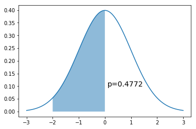
x = np.linspace(-3,3,100)
dist = stats.norm(0,1)
a = -2
b = 0
plt.plot(x, dist.pdf(x))
plt.fill_between(np.linspace(a,b,100), dist.pdf(np.linspace(a,b,100)), alpha=0.5)
plt.text(b+0.1, 0.1, 'p=%.4f' % (dist.cdf(b) - dist.cdf(a)), fontsize=14)
pass
[8]:
from scipy.integrate import quad
[9]:
y, err = quad(dist.pdf, a, b)
y
[9]:
0.47724986805182085
If we can sample directly from the target distribution \(N(0,1)\)
[10]:
n = 10000
x = dist.rvs(n)
np.sum((a < x) & (x < b))/n
[10]:
0.4738
If we cannot sample directly from the target distribution \(N(0,1)\) but can evaluate it at any point.
Recall that \(g(x) = \frac{f(x)}{p(x)}\). Since \(p(x)\) is \(U(a, b)\), \(p(x) = \frac{1}{b-a}\). So we want to calculate
[11]:
n = 10000
x = np.random.uniform(a, b, n)
np.mean((b-a)*dist.pdf(x))
[11]:
0.48069595176138846
Intuition for error rate
We will just work this out for a proper integral \(f(x)\) defined in the unit cube and bounded by \(|f(x)| \le 1\). Draw a random uniform vector \(x\) in the unit cube. Then
Now consider summing over many such IID draws \(S_n = f(x_1) + f(x_2) + \cdots + f(x_n)\). We have
and as expected, we see that \(I \approx S_n/n\). From Chebyshev’s inequality,
Suppose we want 1% accuracy and 99% confidence - i.e. set \(\epsilon = \delta = 0.01\). The above inequality tells us that we can achieve this with just \(n = 1/(\delta \epsilon^2) = 1,000,000\) samples, regardless of the data dimensionality.
Example
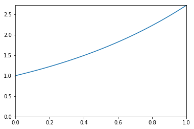
We want to estimate the following integral \(\int_0^1 e^x dx\).
[12]:
x = np.linspace(0, 1, 100)
plt.plot(x, np.exp(x))
plt.xlim([0,1])
plt.ylim([0, np.exp(1)])
pass
Analytic solution
[13]:
from sympy import symbols, integrate, exp

x = symbols('x')
expr = integrate(exp(x), (x,0,1))
expr.evalf()
[13]:
1.71828182845905
Using quadrature
[14]:
from scipy import integrate

y, err = integrate.quad(exp, 0, 1)
y
[14]:
1.7182818284590453
Monte Carlo integration
[15]:
for n in 10**np.array([1,2,3,4,5,6,7,8]):
    x = np.random.uniform(0, 1, n)
    sol = np.mean(np.exp(x))
    print('%10d %.6f' % (n, sol))
        10 1.847075
       100 1.845910
      1000 1.731000
     10000 1.727204
    100000 1.719337
   1000000 1.718142
  10000000 1.718240
 100000000 1.718388
Monitoring variance in Monte Carlo integration
We are often interested in knowing how many iterations it takes for Monte Carlo integration to “converge”. To do this, we would like some estimate of the variance, and it is useful to inspect such plots. One simple way to get confidence intervals for the plot of Monte Carlo estimate against number of iterations is simply to do many such simulations.
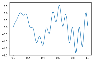
For the example, we will try to estimate the function (again)
[16]:
def f(x):
    return x * np.cos(71*x) + np.sin(13*x)
[17]:
x = np.linspace(0, 1, 100)
plt.plot(x, f(x))
pass
Single MC integration estimate
[18]:
n = 100
x = f(np.random.random(n))
y = 1.0/n * np.sum(x)
y
[18]:
0.03103616434230248
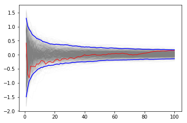
Using multiple independent sequences to monitor convergence
We vary the sample size from 1 to 100 and calculate the value of \(y = \sum{x}/n\) for 1000 replicates. We then plot the 2.5th and 97.5th percentile of the 1000 values of \(y\) to see how the variation in \(y\) changes with sample size. The blue lines indicate the 2.5th and 97.5th percentiles, and the red line a sample path.
[19]:
n = 100
reps = 1000

x = f(np.random.random((n, reps)))
y = 1/np.arange(1, n+1)[:, None] * np.cumsum(x, axis=0)
upper, lower = np.percentile(y, [2.5, 97.5], axis=1)
[20]:
plt.plot(np.arange(1, n+1), y, c='grey', alpha=0.02)
plt.plot(np.arange(1, n+1), y[:, 0], c='red', linewidth=1);
plt.plot(np.arange(1, n+1), upper, 'b', np.arange(1, n+1), lower, 'b')
pass
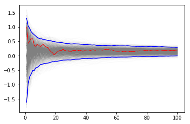
Using bootstrap to monitor convergence
If it is too expensive to do 1000 replicates, we can use a bootstrap instead.
[21]:
xb = np.random.choice(x[:,0], (n, reps), replace=True)
yb = 1/np.arange(1, n+1)[:, None] * np.cumsum(xb, axis=0)
upper, lower = np.percentile(yb, [2.5, 97.5], axis=1)
[22]:
plt.plot(np.arange(1, n+1)[:, None], yb, c='grey', alpha=0.02)
plt.plot(np.arange(1, n+1), yb[:, 0], c='red', linewidth=1)
plt.plot(np.arange(1, n+1), upper, 'b', np.arange(1, n+1), lower, 'b')
pass
Variance Reduction
With independent samples, the variance of the Monte Carlo estimate is
where \(Y_i = f(x_i)/p(x_i)\). In general, we want to make \(\text{Var}[\bar{g_n}]\) as small as possible for the same number of samples. There are several variance reduction techniques (also colorfully known as Monte Carlo swindles) that have been described - we illustrate the change of variables and importance sampling techniques here.
Change of variables
The Cauchy distribution is given by
Suppose we want to integrate the tail probability \(P(X > 3)\) using Monte Carlo. One way to do this is to draw many samples form a Cauchy distribution, and count how many of them are greater than 3, but this is extremely inefficient.
Only 10% of samples will be used
[23]:
import scipy.stats as stats

h_true = 1 - stats.cauchy().cdf(3)
h_true
[23]:
0.10241638234956674
[24]:
n = 100

x = stats.cauchy().rvs(n)
h_mc = 1.0/n * np.sum(x > 3)
h_mc, np.abs(h_mc - h_true)/h_true
[24]:
(0.13, 0.26932817794994063)
A change of variables lets us use 100% of draws
We are trying to estimate the quantity
Using the substitution \(y = 3/x\) (and a little algebra), we get
Hence, a much more efficient MC estimator is
where \(y_i \sim \mathcal{U}(0, 1)\).
[25]:
y = stats.uniform().rvs(n)
h_cv = 1.0/n * np.sum(3.0/(np.pi * (9 + y**2)))
h_cv, np.abs(h_cv - h_true)/h_true
[25]:
(0.10219440906830025, 0.002167361082027339)
Importance sampling
Suppose we want to evaluate
where \(h(x)\) is some function and \(p(x)\) is the PDF of \(y\). If it is hard to sample directly from \(p\), we can introduce a new density function \(q(x)\) that is easy to sample from, and write
In other words, we sample from \(h(y)\) where \(y \sim q\) and weight it by the likelihood ratio \(\frac{p(y)}{q(y)}\), estimating the integral as
Sometimes, even if we can sample from \(p\) directly, it is more efficient to use another distribution.
Example
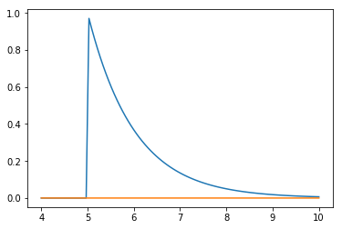
Suppose we want to estimate the tail probability of \(\mathcal{N}(0, 1)\) for \(P(X > 5)\). Regular MC integration using samples from \(\mathcal{N}(0, 1)\) is hopeless since nearly all samples will be rejected. However, we can use the exponential density truncated at 5 as the importance function and use importance sampling. Note that \(h\) here is simply the identify function.
[26]:
x = np.linspace(4, 10, 100)
plt.plot(x, stats.expon(5).pdf(x))
plt.plot(x, stats.norm().pdf(x))
pass
Expected answer
We expect about 3 draws out of 10,000,000 from \(\mathcal{N}(0, 1)\) to have a value greater than 5. Hence simply sampling from \(\mathcal{N}(0, 1)\) is hopelessly inefficient for Monte Carlo integration.
[27]:
%precision 10
[27]:
'%.10f'
[28]:
v_true = 1 - stats.norm().cdf(5)
v_true
[28]:
2.866515719235352e-07
Using direct Monte Carlo integration
[29]:
n = 10000
y = stats.norm().rvs(n)
v_mc = 1.0/n * np.sum(y > 5)
# estimate and relative error
v_mc, np.abs(v_mc - v_true)/v_true
[29]:
(0.0, 1.0)
Using importance sampling
[30]:
n = 10000
y = stats.expon(loc=5).rvs(n)
v_is = 1.0/n * np.sum(stats.norm().pdf(y)/stats.expon(loc=5).pdf(y))
# estimate and relative error
v_is, np.abs(v_is- v_true)/v_true
[30]:
(2.8290057563382236e-07, 0.01308555981236137)
[ ]: