Sparse Matrices
[1]:
%matplotlib inline
import numpy as np
import pandas as pd
from scipy import sparse
import scipy.sparse.linalg as spla
import matplotlib.pyplot as plt
import seaborn as sns
[2]:
sns.set_context('notebook', font_scale=1.5)
Creating a sparse matrix
There are many applications in which we deal with matrices that are mostly zeros. For example, a matrix representing social networks is very sparse - there are 7 billion people, but most people are only connected to a few hundred or thousand others directly. Storing such a social network as a sparse rather than dense matrix will offer orders of magnitude reductions in memory requirements and corresponding speed-ups in computation.
Coordinate format
The simplest sparse matrix format is built from the coordinates and values of the non-zero entries.
From dense matrix
[3]:
A = np.random.poisson(0.2, (5,15)) * np.random.randint(0, 10, (5, 15))
A
[3]:
array([[9, 0, 0, 0, 0, 0, 4, 0, 0, 0, 0, 0, 0, 0, 0],
       [0, 0, 0, 0, 0, 0, 0, 0, 0, 0, 4, 0, 8, 0, 0],
       [0, 0, 9, 0, 0, 0, 0, 0, 0, 0, 0, 0, 0, 8, 0],
       [0, 0, 0, 0, 0, 0, 0, 0, 0, 0, 0, 0, 0, 5, 0],
       [0, 0, 0, 1, 0, 0, 6, 0, 0, 0, 0, 0, 0, 0, 0]])
[4]:
rows, cols = np.nonzero(A)
vals = A[rows, cols]
[5]:
vals
[5]:
array([9, 4, 4, 8, 9, 8, 5, 1, 6])
[6]:
rows
[6]:
array([0, 0, 1, 1, 2, 2, 3, 4, 4])
[7]:
cols
[7]:
array([ 0, 6, 10, 12, 2, 13, 13, 3, 6])
[8]:
X1 = sparse.coo_matrix(A)
X1
[8]:
<5x15 sparse matrix of type '<class 'numpy.int64'>'
        with 9 stored elements in COOrdinate format>
[9]:
print(X1)
  (0, 0)        9
  (0, 6)        4
  (1, 10)       4
  (1, 12)       8
  (2, 2)        9
  (2, 13)       8
  (3, 13)       5
  (4, 3)        1
  (4, 6)        6
From coordinates
Note that the (values, (rows, cols)) argument is a single tuple.
[10]:
X2 = sparse.coo_matrix((vals, (rows, cols)))
X2
[10]:
<5x14 sparse matrix of type '<class 'numpy.int64'>'
        with 9 stored elements in COOrdinate format>
[11]:
print(X2)
  (0, 0)        9
  (0, 6)        4
  (1, 10)       4
  (1, 12)       8
  (2, 2)        9
  (2, 13)       8
  (3, 13)       5
  (4, 3)        1
  (4, 6)        6
Convert back to dense matrix
[12]:
X2.todense()
[12]:
matrix([[9, 0, 0, 0, 0, 0, 4, 0, 0, 0, 0, 0, 0, 0],
        [0, 0, 0, 0, 0, 0, 0, 0, 0, 0, 4, 0, 8, 0],
        [0, 0, 9, 0, 0, 0, 0, 0, 0, 0, 0, 0, 0, 8],
        [0, 0, 0, 0, 0, 0, 0, 0, 0, 0, 0, 0, 0, 5],
        [0, 0, 0, 1, 0, 0, 6, 0, 0, 0, 0, 0, 0, 0]])
Compressed Sparse Row and Column formats
When we have repeated entries in the rows or cols, we can remove the redundancy by indicating the location of the first occurrence of a value and its increment instead of the full coordinates. These are known as CSR or CSC formats.
[13]:
np.vstack([rows, cols])
[13]:
array([[ 0,  0,  1,  1,  2,  2,  3,  4,  4],
       [ 0,  6, 10, 12,  2, 13, 13,  3,  6]])
[14]:
indptr = np.r_[np.searchsorted(rows, np.unique(rows)), len(rows)]
indptr
[14]:
array([0, 2, 4, 6, 7, 9])
[15]:
X3 = sparse.csr_matrix((vals, cols, indptr))
X3
[15]:
<5x14 sparse matrix of type '<class 'numpy.int64'>'
        with 9 stored elements in Compressed Sparse Row format>
[16]:
print(X3)
  (0, 0)        9
  (0, 6)        4
  (1, 10)       4
  (1, 12)       8
  (2, 2)        9
  (2, 13)       8
  (3, 13)       5
  (4, 3)        1
  (4, 6)        6
[17]:
X3.todense()
[17]:
matrix([[9, 0, 0, 0, 0, 0, 4, 0, 0, 0, 0, 0, 0, 0],
        [0, 0, 0, 0, 0, 0, 0, 0, 0, 0, 4, 0, 8, 0],
        [0, 0, 9, 0, 0, 0, 0, 0, 0, 0, 0, 0, 0, 8],
        [0, 0, 0, 0, 0, 0, 0, 0, 0, 0, 0, 0, 0, 5],
        [0, 0, 0, 1, 0, 0, 6, 0, 0, 0, 0, 0, 0, 0]])
Because the coordinate format is more intuitive, it is often more convenient to first create a COO matrix then cast to CSR or CSC form.
[18]:
X4 = X2.tocsr()
[19]:
X4
[19]:
<5x14 sparse matrix of type '<class 'numpy.int64'>'
        with 9 stored elements in Compressed Sparse Row format>
COO summation convention
When entries are repeated in a sparse matrix, they are summed. This provides a quick way to construct confusion matrices for evaluation of multi-class classification algorithms.
[20]:
rows = np.repeat([0,1], 4)
cols = np.repeat([0,1], 4)
vals = np.arange(8)
[21]:
rows
[21]:
array([0, 0, 0, 0, 1, 1, 1, 1])
[22]:
cols
[22]:
array([0, 0, 0, 0, 1, 1, 1, 1])
[23]:
vals
[23]:
array([0, 1, 2, 3, 4, 5, 6, 7])
[24]:
X5 = sparse.coo_matrix((vals, (rows, cols)))
[25]:
X5.todense()
[25]:
matrix([[ 6,  0],
        [ 0, 22]])
[26]:
obs = np.random.randint(0, 2, 100)
pred = np.random.randint(0, 2, 100)
vals = np.ones(100).astype('int')
[27]:
obs
[27]:
array([1, 1, 0, 1, 0, 0, 0, 1, 0, 1, 1, 1, 0, 1, 1, 1, 0, 0, 0, 1, 0, 1,
       1, 0, 0, 0, 1, 0, 1, 1, 0, 0, 0, 1, 1, 1, 0, 0, 0, 0, 0, 0, 0, 1,
       0, 0, 1, 0, 1, 1, 0, 1, 1, 1, 0, 1, 0, 0, 1, 0, 1, 1, 0, 1, 0, 0,
       1, 1, 1, 1, 1, 1, 1, 0, 0, 0, 1, 0, 1, 1, 0, 0, 0, 1, 1, 1, 0, 0,
       1, 0, 0, 0, 1, 0, 0, 0, 0, 0, 1, 0])
[28]:
pred
[28]:
array([0, 0, 1, 0, 1, 1, 1, 0, 0, 1, 1, 0, 0, 1, 0, 1, 0, 0, 0, 1, 1, 0,
       1, 0, 1, 0, 1, 1, 0, 1, 1, 1, 1, 0, 0, 0, 0, 1, 0, 0, 1, 0, 1, 0,
       0, 0, 0, 0, 0, 0, 1, 1, 0, 0, 0, 1, 0, 0, 0, 1, 1, 1, 0, 0, 1, 0,
       1, 1, 0, 1, 1, 1, 1, 0, 1, 0, 0, 1, 0, 1, 0, 1, 0, 0, 0, 0, 0, 0,
       1, 1, 1, 0, 1, 1, 0, 1, 1, 1, 0, 1])
[29]:
vals.shape, obs.shape , pred.shape
[29]:
((100,), (100,), (100,))
[30]:
X6 = sparse.coo_matrix((vals, (pred, obs)))
[31]:
X6.todense()
[31]:
matrix([[27, 26],
        [26, 21]])
For classifications with a large number of classes (e.g. image segmentation), the savings are even more dramatic.
[32]:
from sklearn import datasets
from sklearn.model_selection import train_test_split
from sklearn.neighbors import KNeighborsClassifier
[33]:
iris = datasets.load_iris()
[34]:
knn = KNeighborsClassifier()
X_train, X_test, y_train, y_test = train_test_split(iris.data, iris.target,
                                                    test_size=0.5, random_state=42)
[35]:
pred = knn.fit(X_train, y_train).predict(X_test)
[36]:
pred
[36]:
array([1, 0, 2, 1, 1, 0, 1, 2, 1, 1, 2, 0, 0, 0, 0, 1, 2, 1, 1, 2, 0, 1,
       0, 2, 2, 2, 2, 2, 0, 0, 0, 0, 1, 0, 0, 2, 1, 0, 0, 0, 2, 1, 1, 0,
       0, 1, 1, 2, 1, 2, 1, 2, 1, 0, 2, 1, 0, 0, 0, 1, 1, 0, 0, 0, 1, 0,
       1, 2, 0, 1, 2, 0, 1, 2, 1])
[37]:
y_test
[37]:
array([1, 0, 2, 1, 1, 0, 1, 2, 1, 1, 2, 0, 0, 0, 0, 1, 2, 1, 1, 2, 0, 2,
       0, 2, 2, 2, 2, 2, 0, 0, 0, 0, 1, 0, 0, 2, 1, 0, 0, 0, 2, 1, 1, 0,
       0, 1, 2, 2, 1, 2, 1, 2, 1, 0, 2, 1, 0, 0, 0, 1, 2, 0, 0, 0, 1, 0,
       1, 2, 0, 1, 2, 0, 2, 2, 1])
[38]:
X7 = sparse.coo_matrix((np.ones(len(pred)).astype('int'), (pred, y_test)))
pd.DataFrame(X7.todense(), index=iris.target_names, columns=iris.target_names)
[38]:
| setosa | versicolor | virginica | |
|---|---|---|---|
| setosa | 29 | 0 | 0 |
| versicolor | 0 | 23 | 4 |
| virginica | 0 | 0 | 19 |
[39]:
X7.todense()
[39]:
matrix([[29,  0,  0],
        [ 0, 23,  4],
        [ 0,  0, 19]])
Solving large sparse linear systems
SciPy provides efficient routines for solving large sparse systems as for dense matrices. We will illustrate by calculating the page rank for airports using data from the Bureau of Transportation Statisitcs. The PageRank algorithm is used to rank web pages for search results, but it can be used to rank any node in a directed graph (here we have airports instead of web pages). PageRank is fundamentally about finding the steady state in a Markov chain and can be solved as a linear system.
The update at each time step for the page rank \(PR\) of a page \(p_i\) is

The PageRank algorithm assumes that every node can be reached from every other node. To guard against case where a node has out-degree 0, we allow every node a small random chance of transitioning to any other node using a damping factor \(R\). Then we solve the linear system to find the pagerank score \(R\).

In matrix notation, this is

At steady state,

and we can rearrange terms to solve for \(R\)

[40]:
data = pd.read_csv('../data/airports.csv', usecols=[0,1])
[41]:
data.shape
[41]:
(445827, 2)
[42]:
data.head()
[42]:
| ORIGIN_AIRPORT_ID | DEST_AIRPORT_ID | |
|---|---|---|
| 0 | 10135 | 10397 |
| 1 | 10135 | 10397 |
| 2 | 10135 | 10397 |
| 3 | 10135 | 10397 |
| 4 | 10135 | 10397 |
[43]:
lookup = pd.read_csv('../data/names.csv', index_col=0)
[44]:
lookup.shape
[44]:
(6404, 1)
[45]:
lookup.head()
[45]:
| Description | |
|---|---|
| Code | |
| 10001 | Afognak Lake, AK: Afognak Lake Airport |
| 10003 | Granite Mountain, AK: Bear Creek Mining Strip |
| 10004 | Lik, AK: Lik Mining Camp |
| 10005 | Little Squaw, AK: Little Squaw Airport |
| 10006 | Kizhuyak, AK: Kizhuyak Bay |
[46]:
import networkx as nx
[47]:
g = nx.from_pandas_edgelist(data, source='ORIGIN_AIRPORT_ID', target='DEST_AIRPORT_ID')
[48]:
airports = np.array(g.nodes())
adj_matrix = nx.to_scipy_sparse_matrix(g)
[49]:
out_degrees = np.ravel(adj_matrix.sum(axis=1))
diag_matrix = sparse.diags(1 / out_degrees).tocsr()
M = (diag_matrix @ adj_matrix).T
[50]:
n = len(airports)
d = 0.85
I = sparse.eye(n, format='csc')
A = I - d * M
b = (1-d) / n * np.ones(n) # so the sum of all page ranks is 1
[51]:
A.todense()
[51]:
matrix([[ 1.        , -0.00537975, -0.0085    , ...,  0.        ,
          0.        ,  0.        ],
        [-0.28333333,  1.        , -0.0085    , ...,  0.        ,
          0.        ,  0.        ],
        [-0.28333333, -0.00537975,  1.        , ...,  0.        ,
          0.        ,  0.        ],
        ...,
        [ 0.        ,  0.        ,  0.        , ...,  1.        ,
          0.        ,  0.        ],
        [ 0.        ,  0.        ,  0.        , ...,  0.        ,
          1.        ,  0.        ],
        [ 0.        ,  0.        ,  0.        , ...,  0.        ,
          0.        ,  1.        ]])
[52]:
from scipy.sparse.linalg import spsolve
[53]:
r =  spsolve(A, b)
r.sum()
[53]:
0.9999999999999998
[54]:
idx = np.argsort(r)
[55]:
top10 = idx[-10:][::-1]
bot10 = idx[:10]
[56]:
df = lookup.loc[airports[top10]]
df['degree'] = out_degrees[top10]
df['pagerank']= r[top10]
df
[56]:
| Description | degree | pagerank | |
|---|---|---|---|
| Code | |||
| 10397 | Atlanta, GA: Hartsfield-Jackson Atlanta Intern... | 158 | 0.043286 |
| 13930 | Chicago, IL: Chicago O'Hare International | 139 | 0.033956 |
| 11292 | Denver, CO: Denver International | 129 | 0.031434 |
| 11298 | Dallas/Fort Worth, TX: Dallas/Fort Worth Inter... | 108 | 0.027596 |
| 13487 | Minneapolis, MN: Minneapolis-St Paul Internati... | 108 | 0.027511 |
| 12266 | Houston, TX: George Bush Intercontinental/Houston | 110 | 0.025967 |
| 11433 | Detroit, MI: Detroit Metro Wayne County | 100 | 0.024738 |
| 14869 | Salt Lake City, UT: Salt Lake City International | 78 | 0.019298 |
| 14771 | San Francisco, CA: San Francisco International | 76 | 0.017820 |
| 14107 | Phoenix, AZ: Phoenix Sky Harbor International | 79 | 0.017000 |
[57]:
df = lookup.loc[airports[bot10]]
df['degree'] = out_degrees[bot10]
df['pagerank']= r[bot10]
df
[57]:
| Description | degree | pagerank | |
|---|---|---|---|
| Code | |||
| 14025 | Plattsburgh, NY: Plattsburgh International | 1 | 0.000693 |
| 12265 | Niagara Falls, NY: Niagara Falls International | 1 | 0.000693 |
| 16218 | Yuma, AZ: Yuma MCAS/Yuma International | 1 | 0.000693 |
| 11695 | Flagstaff, AZ: Flagstaff Pulliam | 1 | 0.000693 |
| 14905 | Santa Maria, CA: Santa Maria Public/Capt. G. A... | 1 | 0.000710 |
| 14487 | Redding, CA: Redding Municipal | 1 | 0.000710 |
| 13964 | North Bend/Coos Bay, OR: Southwest Oregon Regi... | 1 | 0.000710 |
| 10157 | Arcata/Eureka, CA: Arcata | 1 | 0.000710 |
| 11049 | College Station/Bryan, TX: Easterwood Field | 1 | 0.000711 |
| 12177 | Hobbs, NM: Lea County Regional | 1 | 0.000711 |
[58]:
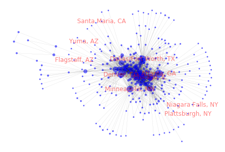
labels = {airports[i]: lookup.loc[airports[i]].str.split(':').str[0].values[0]
          for i in np.r_[top10[:5], bot10[:5]]}
nx.draw(g, pos=nx.spring_layout(g), labels=labels,
        node_color='blue', font_color='red', alpha=0.5,
        node_size=np.clip(5000*r, 1, 5000*r), width=0.1)
/Users/cliburn/opt/anaconda3/lib/python3.7/site-packages/networkx/drawing/nx_pylab.py:579: MatplotlibDeprecationWarning:
The iterable function was deprecated in Matplotlib 3.1 and will be removed in 3.3. Use np.iterable instead.
  if not cb.iterable(width):
[ ]: