Random Variables
[1]:
%matplotlib inline
import itertools as it
import re
import matplotlib.pyplot as plt
import numpy as np
import scipy
from scipy import stats
import toolz as tz
[2]:
import seaborn as sns
from numba import jit
Why are random numbers useful?
If we can draw an arbitrary number of random deviates from a distribution, in some sense, we know everything there is to know about the distribution.
Where do random numbers in the computer come from?
While psuedorandom numbers are generated by a deterministic algorithm, we can mostly treat them as if they were true random numbers and we will drop the “pseudo” prefix. Fundamentally, the algorithm generates random integers which are then normalized to give a floating point number from the standard uniform distribution. Random numbers from other distributions are in turn generated using these uniform random deviates, either via general (inverse transform, accept/reject, mixture representations) or specialized ad-hoc (e.g. Box-Muller) methods.
Generating standard uniform random numbers
Linear congruential generators (LCG)
\(z_{i+1} = (az_i + c) \mod m\)
Hull-Dobell Theorem: The LCG will have a full period for all seeds if and only if
\(c\) and \(m\) are relatively prime,
\(a - 1\) is divisible by all prime factors of \(m\)
\(a - 1\) is a multiple of 4 if \(m\) is a multiple of 4.
The number \(z_0\) is called the seed, and setting it allows us to have a reproducible sequence of “random” numbers. The LCG is typically coded to return \(z/m\), a floating point number in (0, 1). This can be scaled to any other range \((a, b)\).
Note that most PRNGs now use the Mersenne twister, but the LCG is presented because the LCG code much easier to understand and all we hope for is some appreciation for how apparently random sequences can be generated from a deterministic iterative scheme.
[3]:
def lcg(m=2**32, a=1103515245, c=12345):
    lcg.current = (a*lcg.current + c) % m
    return lcg.current/m
[4]:
# setting the seed
lcg.current = 1
[5]:
[lcg() for i in range(10)]
[5]:
[0.25693503906950355,
 0.5878706516232342,
 0.15432575810700655,
 0.767266943352297,
 0.9738139626570046,
 0.5858681506942958,
 0.8511155843734741,
 0.6132153405342251,
 0.7473867232911289,
 0.06236015981994569]
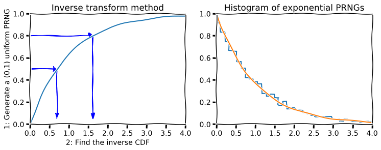
Inverse transform method
Once we have standard uniform numbers, we can often generate random numbers from other distribution using the inverse transform method. Recall that if \(X\) is a continuous random variable with CDF \(F_X\), then \(Y = F_X(X)\) has the standard uniform distribution. Inverting this suggests that if \(Y\) comes from a standard uniform distribution, then \(F_X^{-1}(Y)\) has the same distribution as \(X\). The inverse transform method is used below to generate random numbers from the exponential distribution.
[6]:
def expon_pdf(x, lmabd=1):
    """PDF of exponential distribution."""
    return lmabd*np.exp(-lmabd*x)

def expon_cdf(x, lambd=1):
    """CDF of exponetial distribution."""
    return 1 - np.exp(-lambd*x)

def expon_icdf(p, lambd=1):
    """Inverse CDF of exponential distribution - i.e. quantile function."""
    return -np.log(1-p)/lambd
[7]:
import scipy.stats as stats

dist = stats.expon()
x = np.linspace(0,4,100)
y = np.linspace(0,1,100)

with plt.xkcd():
    plt.figure(figsize=(12,4))
    plt.subplot(121)
    plt.plot(x, expon_cdf(x))
    plt.axis([0, 4, 0, 1])
    for q in [0.5, 0.8]:
        plt.arrow(0, q, expon_icdf(q)-0.1, 0, head_width=0.05, head_length=0.1, fc='b', ec='b')
        plt.arrow(expon_icdf(q), q, 0, -q+0.1, head_width=0.1, head_length=0.05, fc='b', ec='b')
    plt.ylabel('1: Generate a (0,1) uniform PRNG')
    plt.xlabel('2: Find the inverse CDF')
    plt.title('Inverse transform method');

    plt.subplot(122)
    u = np.random.random(10000)
    v = expon_icdf(u)
    plt.hist(v, histtype='step', bins=100, density=True, linewidth=2)
    plt.plot(x, expon_pdf(x), linewidth=2)
    plt.axis([0,4,0,1])
    plt.title('Histogram of exponential PRNGs');
findfont: Font family ['xkcd', 'xkcd Script', 'Humor Sans', 'Comic Sans MS'] not found. Falling back to DejaVu Sans.
findfont: Font family ['xkcd', 'xkcd Script', 'Humor Sans', 'Comic Sans MS'] not found. Falling back to DejaVu Sans.
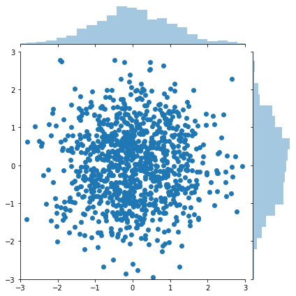
Box-Muller for generating normally distributed random numbers
The Box-Muller transform starts with 2 random uniform numbers \(u\) and \(v\) - Generate an exponentially distributed variable \(r^2\) from \(u\) using the inverse transform method - This means that \(r\) is an exponentially distributed variable on \((0, \infty)\) - Generate a variable \(\theta\) uniformly distributed on \((0, 2\pi)\) from \(v\) by scaling - In polar coordinates, the vector \((r, \theta)\) has an independent bivariate normal distribution - Hence the projection onto the \(x\) and \(y\) axes give independent univariate normal random numbers
Note:
Normal random numbers can also be generated using the general inverse transform method (e.g. by approximating the inverse CDF with a polynomial) or the rejection method (e.g. using the exponential distribution as the sampling distribution).
There is also a variant of Box-Muller that does not require the use of (expensive) trigonometric calculations.
[8]:
n = 1000
u1 = np.random.random(n)
u2 = np.random.random(n)
r_squared = -2*np.log(u1)
r = np.sqrt(r_squared)
theta = 2*np.pi*u2
x = r*np.cos(theta)
y = r*np.sin(theta)
[9]:
g = sns.jointplot(x, y, kind='scatter', xlim=(-3,3), ylim=(-3,3))
pass
Generate univariate random normal deviates
[10]:
@jit(nopython=True)
def box_muller(n):
    """Generate n random normal deviates."""

    u1 = np.random.random((n+1)//2)
    u2 = np.random.random((n+1)//2)
    r_squared = -2*np.log(u1)
    r = np.sqrt(r_squared)
    theta = 2*np.pi*u2
    x = r*np.cos(theta)
    y = r*np.sin(theta)
    z = np.empty(n)
    z[:((n+1)//2)] = x
    z[((n+1)//2):] = y
    return z[:n]
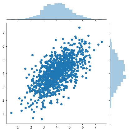
Generating multivariate normal random deviates
[11]:
@jit(nopython=True)
def mvn(mu, sigma, n=1):
    """Generate n samples from multivarate normal with mean mu and covariance sigma."""

    A = np.linalg.cholesky(sigma)
    p = len(mu)

    zs = np.zeros((n, p))
    for i in range(n):
        z = box_muller(p)
        zs[i] = mu + A@z
    return zs
[12]:
mu = 4.0*np.ones(2)
sigma = np.array([[1,0.6], [0.6, 1]])
[13]:
n = 1000
x, y = mvn(mu, sigma, n).T
g = sns.jointplot(x, y, kind='scatter')
pass
[14]:
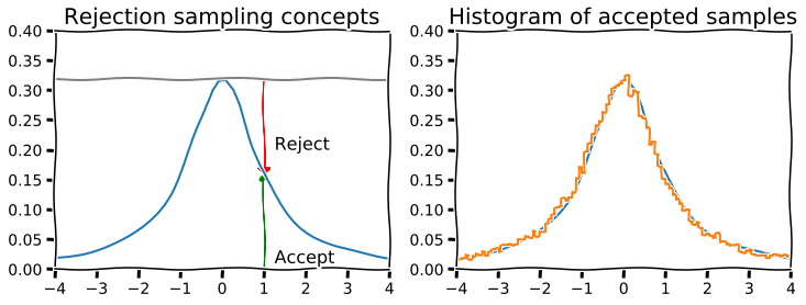
## Rejection sampling
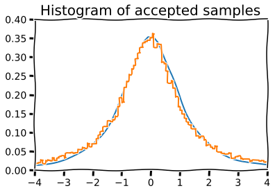
[15]:
# Suppose we want to sample from the truncated Cauchy distribution
# We use the uniform as a proposal distibution (highly inefficient)

x = np.linspace(-4, 4)

dist = stats.cauchy()
upper = dist.pdf(0)

with plt.xkcd():
    plt.figure(figsize=(12,4))
    plt.subplot(121)
    plt.plot(x, dist.pdf(x))
    plt.axhline(upper, color='grey')
    px = 1.0
    plt.arrow(px,0,0,dist.pdf(1.0)-0.01, linewidth=1,
              head_width=0.2, head_length=0.01, fc='g', ec='g')
    plt.arrow(px,upper,0,-(upper-dist.pdf(px)-0.01), linewidth=1,
              head_width=0.3, head_length=0.01, fc='r', ec='r')
    plt.text(px+.25, 0.2, 'Reject', fontsize=16)
    plt.text(px+.25, 0.01, 'Accept', fontsize=16)
    plt.axis([-4,4,0,0.4])
    plt.title('Rejection sampling concepts', fontsize=20)

    plt.subplot(122)
    n = 100000
    # generate from sampling distribution
    u = np.random.uniform(-4, 4, n)
    # accept-reject criterion for each point in sampling distribution
    r = np.random.uniform(0, upper, n)
    # accepted points will come from target (Cauchy) distribution
    v = u[r < dist.pdf(u)]

    plt.plot(x, dist.pdf(x), linewidth=2)

    # Plot scaled histogram
    factor = dist.cdf(4) - dist.cdf(-4)
    hist, bin_edges = np.histogram(v, bins=100, normed=True)
    bin_centers = (bin_edges[:-1] + bin_edges[1:]) / 2.
    plt.step(bin_centers, factor*hist, linewidth=2)

    plt.axis([-4,4,0,0.4])
    plt.title('Histogram of accepted samples', fontsize=20);
/opt/conda/lib/python3.6/site-packages/ipykernel_launcher.py:37: VisibleDeprecationWarning: Passing `normed=True` on non-uniform bins has always been broken, and computes neither the probability density function nor the probability mass function. The result is only correct if the bins are uniform, when density=True will produce the same result anyway. The argument will be removed in a future version of numpy.
findfont: Font family ['xkcd', 'xkcd Script', 'Humor Sans', 'Comic Sans MS'] not found. Falling back to DejaVu Sans.
findfont: Font family ['xkcd', 'xkcd Script', 'Humor Sans', 'Comic Sans MS'] not found. Falling back to DejaVu Sans.
Mixture representations
Sometimes, the target distribution from which we need to generate random numbers can be expressed as a mixture of “simpler” distributions that we already know how to sample from
For example, if \(y\) is drawn from the \(\chi_\nu^2\) distribution, then \(\mathcal{N}(0, \nu/y)\) is a sample from the Student’s T distribution with \(\nu\) degrees of freedom.
[16]:
n = 10000
df = 2
dist = stats.t(df=df)
y = stats.chi2(df=df).rvs(n)
r = stats.norm(0, df/y).rvs(n)

with plt.xkcd():
    plt.plot(x, dist.pdf(x), linewidth=2)

    # Plot scaled histogram
    factor = dist.cdf(4) - dist.cdf(-4)
    hist, bin_edges = np.histogram(v, bins=100, normed=True)
    bin_centers = (bin_edges[:-1] + bin_edges[1:]) / 2.
    plt.step(bin_centers, factor*hist, linewidth=2)

    plt.axis([-4,4,0,0.4])
    plt.title('Histogram of accepted samples', fontsize=20);
/opt/conda/lib/python3.6/site-packages/ipykernel_launcher.py:12: VisibleDeprecationWarning: Passing `normed=True` on non-uniform bins has always been broken, and computes neither the probability density function nor the probability mass function. The result is only correct if the bins are uniform, when density=True will produce the same result anyway. The argument will be removed in a future version of numpy.
  if sys.path[0] == '':
Using numpy.random
Setting seed for reproducibility
[17]:
np.random.seed(123)
Standard uniform
[18]:
np.random.rand(3,4)
[18]:
array([[0.69646919, 0.28613933, 0.22685145, 0.55131477],
       [0.71946897, 0.42310646, 0.9807642 , 0.68482974],
       [0.4809319 , 0.39211752, 0.34317802, 0.72904971]])
Standard normal
[19]:
np.random.randn(3, 4)
[19]:
array([[-0.67888615, -0.09470897,  1.49138963, -0.638902  ],
       [-0.44398196, -0.43435128,  2.20593008,  2.18678609],
       [ 1.0040539 ,  0.3861864 ,  0.73736858,  1.49073203]])
Parameterized distributions
Parameterized distribution functions typically have one or more of location, scale, shape or other parameters that can be specified.
Continuous distributions
[20]:
np.random.uniform(low=-1, high=1, size=(3, 4))
[20]:
array([[ 0.44488677, -0.35408217, -0.27642269, -0.54347354],
       [-0.41257191,  0.26195225, -0.81579012, -0.13259765],
       [-0.13827447, -0.0126298 , -0.14833942, -0.37547755]])
[21]:
np.random.normal(loc=100, scale=15, size=(3, 4))
[21]:
array([[113.91193648,  97.39546476, 100.04268874, 110.32334067],
       [ 86.80695485, 104.25440986,  87.91950223,  74.08495759],
       [ 94.13650309, 108.60708794, 105.07883576,  99.82254258]])
[22]:
np.random.standard_t(df=3, size=(3,4))
[22]:
array([[ 2.26603603,  0.26443366, -2.62014171,  0.73989909],
       [ 0.52766961,  0.84688526, -0.63048839, -0.92233841],
       [ 1.15114019,  0.67780629,  0.82852178,  0.30139753]])
[23]:
np.random.beta(a=0.5, b=0.5, size=(10,))
[23]:
array([0.9853416 , 0.36941327, 0.17888099, 0.42376794, 0.12553194,
       0.32966061, 0.37205691, 0.39564619, 0.19150945, 0.83135736])
Discrete distributions
[24]:
np.random.poisson(lam=10, size=(10,))
[24]:
array([ 8, 8, 11, 15, 8, 7, 13, 12, 9, 9])
[25]:
np.random.binomial(n=10, p=0.6, size=(10,))
[25]:
array([8, 7, 4, 6, 6, 5, 5, 8, 5, 4])
[26]:
np.random.negative_binomial(n=10, p=0.6, size=(10,))
[26]:
array([10, 8, 3, 0, 6, 6, 4, 6, 3, 5])
[27]:
np.random.geometric(p=0.6, size=(10,))
[27]:
array([2, 1, 1, 5, 1, 1, 1, 4, 1, 2])
Multivariate distributions
[28]:
np.random.multinomial(4, [0.1, 0.2, 0.3, 0.4], size=5)
[28]:
array([[1, 0, 1, 2],
       [1, 0, 1, 2],
       [2, 1, 1, 0],
       [0, 0, 2, 2],
       [0, 3, 0, 1]])
[29]:
np.random.multivariate_normal([10, 10], np.array([[3, 0.5], [0.5, 2]]), 5)
[29]:
array([[12.36034662, 10.17775889],
       [10.59100147,  9.72067176],
       [ 9.14425098,  7.58936076],
       [12.13627781,  8.89252357],
       [11.98365842, 11.00145391]])
Sampling with and without replacement
[30]:
# Sampling is done with replacement by default
np.random.choice(4, 12)
[30]:
array([1, 0, 1, 1, 0, 3, 0, 0, 0, 0, 2, 0])
[31]:
# Probability weights can be given
np.random.choice(4, 12, p=[.4, .1, .1, .4])
[31]:
array([0, 3, 0, 3, 3, 3, 3, 3, 1, 3, 0, 3])
[32]:
x = np.random.randint(0, 10, (8, 12))
x
[32]:
array([[7, 3, 1, 3, 9, 3, 6, 2, 3, 1, 9, 8],
       [0, 2, 3, 7, 9, 2, 7, 9, 7, 1, 4, 7],
       [4, 7, 8, 0, 2, 7, 4, 3, 7, 3, 7, 0],
       [7, 6, 8, 6, 8, 0, 5, 3, 2, 4, 3, 3],
       [9, 7, 1, 8, 0, 1, 4, 7, 2, 4, 8, 3],
       [4, 9, 6, 2, 7, 7, 7, 4, 7, 8, 4, 0],
       [7, 6, 3, 4, 1, 1, 7, 2, 7, 8, 9, 4],
       [4, 4, 7, 7, 9, 9, 4, 1, 5, 5, 8, 9]])
[33]:
# sampling individual elements
np.random.choice(x.ravel(), 12)
[33]:
array([1, 2, 7, 4, 7, 3, 8, 7, 7, 2, 4, 8])
[34]:
# sampling rows
idx = np.random.choice(x.shape[0], 4)
x[idx, :]
[34]:
array([[9, 7, 1, 8, 0, 1, 4, 7, 2, 4, 8, 3],
       [7, 6, 3, 4, 1, 1, 7, 2, 7, 8, 9, 4],
       [4, 9, 6, 2, 7, 7, 7, 4, 7, 8, 4, 0],
       [7, 6, 8, 6, 8, 0, 5, 3, 2, 4, 3, 3]])
[35]:
# sampling columns
idx = np.random.choice(x.shape[1], 4)
x[:, idx]
[35]:
array([[9, 6, 8, 8],
       [9, 7, 7, 7],
       [2, 4, 0, 0],
       [8, 5, 3, 3],
       [0, 4, 3, 3],
       [7, 7, 0, 0],
       [1, 7, 4, 4],
       [9, 4, 9, 9]])
[36]:
# Give the argument replace=False
try:
    np.random.choice(4, 12, replace=False)
except ValueError as e:
    print(e)
Cannot take a larger sample than population when 'replace=False'
Shuffles, permutations and combinations
Shuffle
Shuffle is an in-place permutation
[37]:
xs = np.arange(10)
xs
[37]:
array([0, 1, 2, 3, 4, 5, 6, 7, 8, 9])
[38]:
np.random.shuffle(xs)
xs
[38]:
array([1, 0, 8, 7, 3, 6, 4, 9, 5, 2])
Shuffle permutes rows of a matrix
[39]:
xs = np.arange(12).reshape(3,4)
xs
[39]:
array([[ 0,  1,  2,  3],
       [ 4,  5,  6,  7],
       [ 8,  9, 10, 11]])
[40]:
np.random.shuffle(xs)
xs
[40]:
array([[ 4,  5,  6,  7],
       [ 8,  9, 10, 11],
       [ 0,  1,  2,  3]])
[41]:
# To shuffle columns instead, transpose before shuffling
np.random.shuffle(x.T)
x
[41]:
array([[1, 3, 2, 3, 9, 7, 1, 8, 3, 9, 3, 6],
       [3, 2, 9, 7, 9, 0, 1, 7, 2, 4, 7, 7],
       [8, 7, 3, 0, 2, 4, 3, 0, 7, 7, 7, 4],
       [8, 6, 3, 6, 8, 7, 4, 3, 0, 3, 2, 5],
       [1, 7, 7, 8, 0, 9, 4, 3, 1, 8, 2, 4],
       [6, 9, 4, 2, 7, 4, 8, 0, 7, 4, 7, 7],
       [3, 6, 2, 4, 1, 7, 8, 4, 1, 9, 7, 7],
       [7, 4, 1, 7, 9, 4, 5, 9, 9, 8, 5, 4]])
Permutation
[42]:
np.random.permutation(10)
[42]:
array([1, 2, 3, 4, 7, 6, 5, 9, 8, 0])
[43]:
# When given an integre n, permutation treats is as the array arange(n)
xs = np.arange(10)
np.random.permutation(xs)
[43]:
array([6, 5, 2, 7, 4, 3, 9, 8, 1, 0])
[44]:
xs = np.arange(12).reshape(3,4)
np.random.permutation(xs)
[44]:
array([[ 0,  1,  2,  3],
       [ 4,  5,  6,  7],
       [ 8,  9, 10, 11]])
[45]:
# Use indices if you needed to shuffle collections of arrays in synchrony
x = np.arange(12).reshape(4,3)
y = x + 10
idx = np.random.permutation(x.shape[0])
list(zip(x[idx, :], y[idx, :]))
[45]:
[(array([0, 1, 2]), array([10, 11, 12])),
 (array([ 9, 10, 11]), array([19, 20, 21])),
 (array([3, 4, 5]), array([13, 14, 15])),
 (array([6, 7, 8]), array([16, 17, 18]))]
Using itertools
[46]:
list(map(lambda x: ''.join(x), it.permutations('abc')))
[46]:
['abc', 'acb', 'bac', 'bca', 'cab', 'cba']
[47]:
list(map(lambda x: ''.join(x), it.combinations('abcd', 3)))
[47]:
['abc', 'abd', 'acd', 'bcd']
[48]:
list(map(lambda x: ''.join(x), it.combinations_with_replacement('abcd', 2)))
[48]:
['aa', 'ab', 'ac', 'ad', 'bb', 'bc', 'bd', 'cc', 'cd', 'dd']
Leave one out
Unlike R, Python does not use negative indexing to delete items. So we need to create a Boolean index to create leave-one-out sequences.
[49]:
x = np.arange(10, 15)
for i in range(len(x)):
    idx = np.arange(len(x)) != i
    print(x[idx])
[11 12 13 14]
[10 12 13 14]
[10 11 13 14]
[10 11 12 14]
[10 11 12 13]
Using scipy.stats
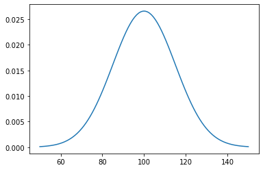
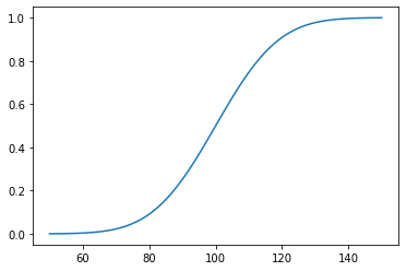
Example: modeling IQ
Suppose IQ is normally distributed with a mean of 0 and a standard deviation of 15.
[50]:
dist = stats.norm(loc=100, scale=15)
Random variates
[51]:
dist.rvs(10)
[51]:
array([102.13638378, 108.11846946, 120.10148055,  76.46115809,
        92.34485689,  93.28342862, 114.06775446,  94.65005408,
        71.5723661 , 101.31595696])
[52]:
xs = np.linspace(50, 150, 100)
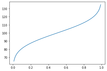
Percentiles
[55]:
cdf = np.linspace(0, 1, 100)
plt.plot(cdf, dist.ppf(cdf))
pass
[56]:
data = np.random.normal(110, 15, 100)
Exercises
1. If your IQ is 138, what percentage of the population has a higher IQ?
[57]:
dist = stats.norm(loc=100, scale=15)
[58]:
100 * (1 - dist.cdf(138))
[58]:
0.564917275556065
Via simulation
[59]:
n = int(1e6)
samples = dist.rvs(n)
[60]:
np.sum(samples > 138)/n
[60]:
0.005694
2. If your IQ is at the 88th percentile, what is your IQ?
[61]:
dist.ppf(0.88)
[61]:
117.62480188099136
Via simulation
[62]:
samples = np.sort(samples)
samples[int(0.88*n)]
[62]:
117.6441801355916
3. What proportion of the population has IQ between 70 and 90?
[63]:
dist.cdf(90) - dist.cdf(70)
[63]:
0.2297424055987437
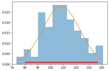
MLE fit and confidence intervals
[65]:
loc, scale = stats.norm.fit(data)
loc, scale
[65]:
(108.25727900498485, 14.374033188248367)
[66]:
dist = stats.norm(loc, scale)
[67]:
xs = np.linspace(data.min(), data.max(), 100)
plt.hist(data, 12, histtype='stepfilled', normed=True, alpha=0.5)
plt.plot(xs, dist.pdf(xs))
plt.plot(dist.interval(0.95), [0.001, 0.001], c='r', linewidth=3)
pass
/opt/conda/lib/python3.6/site-packages/ipykernel_launcher.py:2: MatplotlibDeprecationWarning:
The 'normed' kwarg was deprecated in Matplotlib 2.1 and will be removed in 3.1. Use 'density' instead.
Sampling
Without replication
[68]:
np.random.choice(range(10), 5, replace=False)
[68]:
array([7, 2, 3, 1, 6])
With replication
[69]:
np.random.choice(range(10), 15)
[69]:
array([9, 4, 9, 9, 1, 0, 4, 1, 6, 8, 3, 0, 5, 4, 7])
Example
How often do we get a run of 5 or more consecutive heads in 100 coin tosses if we repeat the experiment 1000 times?
What if the coin is biased to generate heads only 40% of the time?
[70]:
expts = 1000
tosses = 100
We assume that 0 maps to T and 1 to H
[71]:
xs = np.random.choice([0,1], (expts, tosses))
For biased coin
[72]:
ys = np.random.choice([0,1], (expts, tosses), p=[0.6, 0.4])
Using a finite state machine
[73]:
runs = 0
for x in xs:
    m = 0
    for i in x:
        if i == 1:
            m += 1
            if m >=5:
                runs += 1
                break
        else:
            m = 0
runs
[73]:
796
Using partitionby
[74]:
runs = 0
for x in xs:
    parts = tz.partitionby(lambda i: i==1, x)
    for part in parts:
        if part[0] == 1 and len(part) >= 5:
            runs += 1
            break
runs
[74]:
796
Using sliding windows
[75]:
runs = 0
for x in xs:
    for w in tz.sliding_window(5, x):
        if np.sum(w) == 5:
            runs += 1
            break
runs
[75]:
796
Using a regular expression
[76]:
xs = xs.astype('str')
[77]:
runs = 0
for x in xs:
    if (re.search(r'1{5,}', ''.join(x))):
        runs += 1
runs
[77]:
796