Using PyMC3
PyMC3 is a Python package for doing MCMC using a variety of samplers, including Metropolis, Slice and Hamiltonian Monte Carlo. See Probabilistic Programming in Python using PyMC for a description. The GitHub site also has many examples and links for further exploration.
Note: PyMC4 is based on TensorFlow rather than Theano but will have a similar API so everyghitn learned should be transferable.
! pip install --quiet arviz
! pip install --quiet pymc3
! pip install --quiet daft
! pip install --quiet seaborn
! conda install --yes --quiet mkl-service
[1]:
import warnings

warnings.simplefilter('ignore', UserWarning)
Other resources
Some examples are adapted from:
[2]:
%matplotlib inline
[3]:
import numpy as np
import numpy.random as rng
import matplotlib.pyplot as plt
import seaborn as sns
import pandas as pd
import pymc3 as pm
import scipy.stats as stats
import daft
import arviz as az
WARNING (theano.configdefaults): install mkl with `conda install mkl-service`: No module named 'mkl'
WARNING (theano.tensor.blas): Using NumPy C-API based implementation for BLAS functions.
[4]:
import theano
theano.config.warn.round=False
[5]:
sns.set_context('notebook')
plt.style.use('seaborn-darkgrid')
Introduction to PyMC3
Distributions in pymc3
[6]:
print('\n'.join([d for d in dir(pm.distributions) if d[0].isupper()]))
AR
AR1
Bernoulli
Beta
BetaBinomial
Binomial
Bound
Categorical
Cauchy
ChiSquared
Constant
ConstantDist
Continuous
DensityDist
Dirichlet
Discrete
DiscreteUniform
DiscreteWeibull
Distribution
ExGaussian
Exponential
Flat
GARCH11
Gamma
GaussianRandomWalk
Geometric
Gumbel
HalfCauchy
HalfFlat
HalfNormal
HalfStudentT
Interpolated
InverseGamma
KroneckerNormal
Kumaraswamy
LKJCholeskyCov
LKJCorr
Laplace
Logistic
LogitNormal
Lognormal
MatrixNormal
Mixture
Multinomial
MvGaussianRandomWalk
MvNormal
MvStudentT
MvStudentTRandomWalk
NegativeBinomial
NoDistribution
Normal
NormalMixture
OrderedLogistic
Pareto
Poisson
Rice
Simulator
SkewNormal
StudentT
TensorType
Triangular
TruncatedNormal
Uniform
VonMises
Wald
Weibull
Wishart
WishartBartlett
ZeroInflatedBinomial
ZeroInflatedNegativeBinomial
ZeroInflatedPoisson
[7]:
d = pm.Normal.dist(mu=0, sd=1)
[8]:
d.dist()
[8]:
Random samples
[9]:
d.random(size=5)
[9]:
array([ 0.84368789, -0.2096697 , 0.54824422, -0.25347107, -0.4494888 ])
Log probability
[10]:
d.logp(0).eval()
[10]:
array(-0.91893853)
Custom distributions
The pymc3 algorithms generally only work with the log probability of a distribution. Hence it is easy to define custom distributions to use in your models by providing a logp function.
[11]:
def logp(x, μ=0, σ=1):
    """Normal distribtuion."""
    return -0.5*np.log(2*np.pi) - np.log(σ) - (x-μ)**2/(2*σ**2)
[12]:
d = pm.DensityDist.dist(logp)
[13]:
d.logp(0)
[13]:
-0.9189385332046727
Example: Estimating coin bias
We start with the simplest model - that of determining the bias of a coin from observed outcomes.
Here the prior is a beta distribution with paramters \(a\) and \(b\), the likelihood assumes that the number of heads follows a binomial distribution with parameters \(n\) and \(p\), and we wish to estimate the posterior distribution of \(\theta = p\).
Prior = Beta distribution
[14]:
pars = [(0.5, 0.5), (1,1), (1,10), (5,5), (10, 1), (10,10)]

fig, axes = plt.subplots(2, 3, figsize=(12, 8))
for i, (a, b) in enumerate(pars):
    ax = axes[i // 3, i % 3]
    θ = np.linspace(0, 1, 100)
    dens = stats.beta(a, b).pdf(θ)
    ax.plot(θ, dens)
    ax.set_title('a=%.1f, b=%.1f' % (a, b))

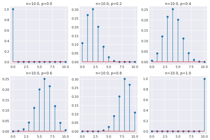
Posterior = bionmial distribution
[15]:
pars = [0, 0.2, 0.4, 0.6, 0.8, 1]
n = 10

fig, axes = plt.subplots(2, 3, figsize=(12, 8))
for i, p in enumerate(pars):
    ax = axes[i // 3, i % 3]
    θ = np.arange(0, n+1)
    dens = stats.binom(n, p).pmf(θ)
    ax.stem(θ, dens)
    ax.set_title('n=%.1f, p=%.1f' % (n, p))
Setting up the model
[16]:
n = 100
heads = 61
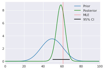
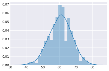
Analytical solution
[17]:
a, b = 10, 10
prior = stats.beta(a, b)
post = stats.beta(heads+a, n-heads+b)
ci = post.interval(0.95)

xs = np.linspace(0, 1, 100)
plt.plot(prior.pdf(xs), label='Prior')
plt.plot(post.pdf(xs), c='green', label='Posterior')
plt.axvline(100*heads/n, c='red', alpha=0.4, label='MLE')
plt.xlim([0, 100])
plt.axhline(0.3, ci[0], ci[1], c='black', linewidth=2, label='95% CI');
plt.legend()
pass
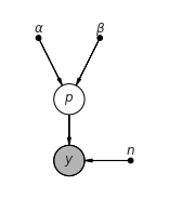
Graphical model
[18]:
pgm = daft.PGM(shape=[2.5, 3.0], origin=[0, -0.5])

pgm.add_node(daft.Node("alpha", r"$\alpha$", 0.5, 2, fixed=True))
pgm.add_node(daft.Node("beta", r"$\beta$", 1.5, 2, fixed=True))
pgm.add_node(daft.Node("p", r"$p$", 1, 1))
pgm.add_node(daft.Node("n", r"$n$", 2, 0, fixed=True))
pgm.add_node(daft.Node("y", r"$y$", 1, 0, observed=True))

pgm.add_edge("alpha", "p")
pgm.add_edge("beta", "p")
pgm.add_edge("n", "y")
pgm.add_edge("p", "y")

pgm.render()
pass
The Model context
When you specify a model, you are adding nodes to a computation graph. When executed, the graph is compiled via Theno. Hence, pymc3 uses the Model context manager to automatically add new nodes.
[19]:
niter = 2000
with pm.Model() as coin_context:
    p = pm.Beta('p', alpha=2, beta=2)
    y = pm.Binomial('y', n=n, p=p, observed=heads)
    trace = pm.sample(niter)
Auto-assigning NUTS sampler...
Initializing NUTS using jitter+adapt_diag...
Multiprocess sampling (4 chains in 4 jobs)
NUTS: [p]
Sampling 4 chains, 0 divergences: 100%|██████████| 10000/10000 [00:02<00:00, 4848.37draws/s]
[20]:
coin_context
[20]:
Under the hood
Theano
Theano builds functions as mathematical expression graphs and compiles them into C for actual computation, making use of GPU resources where available.
Performing calculations in Theano generally follows the following 3 steps (from official docs):
declare variables (a,b) and give their types
build expressions for how to put those variables together
compile expression graphs to functions in order to use them for computation.
[24]:
import theano
import theano.tensor as tt
theano.config.compute_test_value = "off"
This part builds symbolic expressions.
[25]:
a = tt.iscalar('a')
b = tt.iscalar('x')
c = a + b
This step compiles a function whose inputs are [a, b] and outputs are [c].
[26]:
f = theano.function([a, b], [c])
[27]:
f
[27]:
<theano.compile.function_module.Function at 0x7fd287284160>
[28]:
f(3, 4)
[28]:
[array(7, dtype=int32)]
Within a model context,
when you add an unbounded variable, it is defined as a Theano variable and added to the prior part of the log posterior function
when you add a bounded variable, a transformed version is defined as a Theano variable and and added to the log posterior function
The inverse transformation is used to define the original variable - this is a deterministic variable
when you add an observed variable bound to data, the data is added to the likelihood part of the log posterior
See PyMC3 and Theano for details.
[29]:
help(pm.sample)
Help on function sample in module pymc3.sampling:

sample(draws=500, step=None, init='auto', n_init=200000, start=None, trace=None, chain_idx=0, chains=None, cores=None, tune=500, progressbar=True, model=None, random_seed=None, discard_tuned_samples=True, compute_convergence_checks=True, **kwargs)
    Draw samples from the posterior using the given step methods.

    Multiple step methods are supported via compound step methods.

    Parameters
    ----------
    draws : int
        The number of samples to draw. Defaults to 500. The number of tuned samples are discarded
        by default. See ``discard_tuned_samples``.
    init : str
        Initialization method to use for auto-assigned NUTS samplers.

        * auto : Choose a default initialization method automatically.
          Currently, this is ``'jitter+adapt_diag'``, but this can change in the future.
          If you depend on the exact behaviour, choose an initialization method explicitly.
        * adapt_diag : Start with a identity mass matrix and then adapt a diagonal based on the
          variance of the tuning samples. All chains use the test value (usually the prior mean)
          as starting point.
        * jitter+adapt_diag : Same as ``adapt_diag``\, but add uniform jitter in [-1, 1] to the
          starting point in each chain.
        * advi+adapt_diag : Run ADVI and then adapt the resulting diagonal mass matrix based on the
          sample variance of the tuning samples.
        * advi+adapt_diag_grad : Run ADVI and then adapt the resulting diagonal mass matrix based
          on the variance of the gradients during tuning. This is **experimental** and might be
          removed in a future release.
        * advi : Run ADVI to estimate posterior mean and diagonal mass matrix.
        * advi_map: Initialize ADVI with MAP and use MAP as starting point.
        * map : Use the MAP as starting point. This is discouraged.
        * nuts : Run NUTS and estimate posterior mean and mass matrix from the trace.
    step : function or iterable of functions
        A step function or collection of functions. If there are variables without step methods,
        step methods for those variables will be assigned automatically.  By default the NUTS step
        method will be used, if appropriate to the model; this is a good default for beginning
        users.
    n_init : int
        Number of iterations of initializer. Only works for 'nuts' and 'ADVI'.
        If 'ADVI', number of iterations, if 'nuts', number of draws.
    start : dict, or array of dict
        Starting point in parameter space (or partial point)
        Defaults to ``trace.point(-1))`` if there is a trace provided and model.test_point if not
        (defaults to empty dict). Initialization methods for NUTS (see ``init`` keyword) can
        overwrite the default.
    trace : backend, list, or MultiTrace
        This should be a backend instance, a list of variables to track, or a MultiTrace object
        with past values. If a MultiTrace object is given, it must contain samples for the chain
        number ``chain``. If None or a list of variables, the NDArray backend is used.
        Passing either "text" or "sqlite" is taken as a shortcut to set up the corresponding
        backend (with "mcmc" used as the base name).
    chain_idx : int
        Chain number used to store sample in backend. If ``chains`` is greater than one, chain
        numbers will start here.
    chains : int
        The number of chains to sample. Running independent chains is important for some
        convergence statistics and can also reveal multiple modes in the posterior. If ``None``,
        then set to either ``cores`` or 2, whichever is larger.
    cores : int
        The number of chains to run in parallel. If ``None``, set to the number of CPUs in the
        system, but at most 4.
    tune : int
        Number of iterations to tune, defaults to 500. Samplers adjust the step sizes, scalings or
        similar during tuning. Tuning samples will be drawn in addition to the number specified in
        the ``draws`` argument, and will be discarded unless ``discard_tuned_samples`` is set to
        False.
    progressbar : bool
        Whether or not to display a progress bar in the command line. The bar shows the percentage
        of completion, the sampling speed in samples per second (SPS), and the estimated remaining
        time until completion ("expected time of arrival"; ETA).
    model : Model (optional if in ``with`` context)
    random_seed : int or list of ints
        A list is accepted if ``cores`` is greater than one.
    discard_tuned_samples : bool
        Whether to discard posterior samples of the tune interval.
    compute_convergence_checks : bool, default=True
        Whether to compute sampler statistics like Gelman-Rubin and ``effective_n``.

    Returns
    -------
    trace : pymc3.backends.base.MultiTrace
        A ``MultiTrace`` object that contains the samples.

    Notes
    -----
    Optional keyword arguments can be passed to ``sample`` to be delivered to the
    ``step_method``s used during sampling. In particular, the NUTS step method accepts
    a number of arguments. Common options are:

        * target_accept: float in [0, 1]. The step size is tuned such that we approximate this
          acceptance rate. Higher values like 0.9 or 0.95 often work better for problematic
          posteriors.
        * max_treedepth: The maximum depth of the trajectory tree.
        * step_scale: float, default 0.25
          The initial guess for the step size scaled down by :math:`1/n**(1/4)`

    You can find a full list of arguments in the docstring of the step methods.

    Examples
    --------
    .. code:: ipython

        >>> import pymc3 as pm
        ... n = 100
        ... h = 61
        ... alpha = 2
        ... beta = 2

    .. code:: ipython

        >>> with pm.Model() as model: # context management
        ...     p = pm.Beta('p', alpha=alpha, beta=beta)
        ...     y = pm.Binomial('y', n=n, p=p, observed=h)
        ...     trace = pm.sample(2000, tune=1000, cores=4)
        >>> pm.summary(trace)
               mean        sd  mc_error   hpd_2.5  hpd_97.5
        p  0.604625  0.047086   0.00078  0.510498  0.694774
Specifying sampler (step) and multiple chains
[30]:
with coin_context:
    step = pm.Metropolis()
    t = pm.sample(niter, step=step, chains=8, random_seed=123)
Multiprocess sampling (8 chains in 4 jobs)
Metropolis: [p]
Sampling 8 chains, 0 divergences: 100%|██████████| 20000/20000 [00:03<00:00, 5999.39draws/s]
The number of effective samples is smaller than 25% for some parameters.
Samplers available
For continuous distributions, it is hard to beat NUTS and hence this is the default. To learn more, see A Conceptual Introduction to Hamiltonian Monte Carlo.
[31]:
print('\n'.join(m for m in dir(pm.step_methods) if m[0].isupper()))
BinaryGibbsMetropolis
BinaryMetropolis
CategoricalGibbsMetropolis
CauchyProposal
CompoundStep
DEMetropolis
ElemwiseCategorical
EllipticalSlice
HamiltonianMC
LaplaceProposal
Metropolis
MultivariateNormalProposal
NUTS
NormalProposal
PoissonProposal
Slice
Generally, the sampler will be automatically selected based on the type of the variable (discrete or continuous), but there are many samples that you can explicitly specify if you want to learn more about them or understand why an alternative would be better than the default for your problem.
[32]:
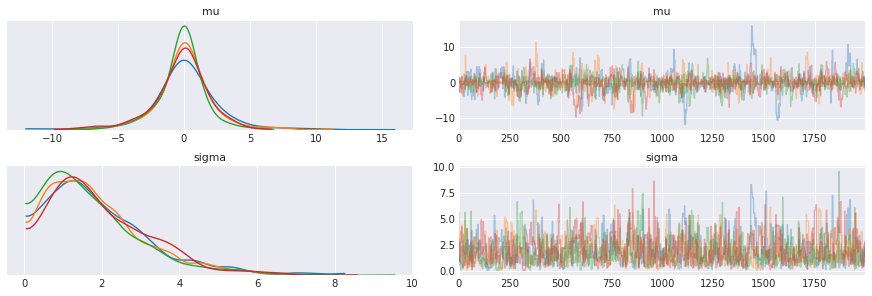
niter = 2000
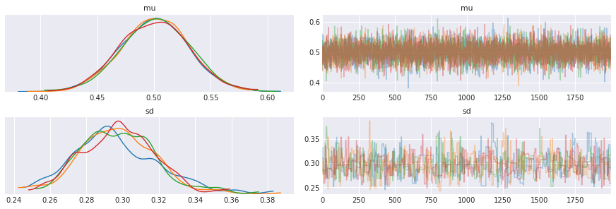
with pm.Model() as normal_context:
mu = pm.Normal('mu', mu=0, sd=100)
sd = pm.HalfCauchy('sd', beta=2)
y = pm.Normal('y', mu=mu, sd=sd, observed=xs)
step1 = pm.Slice(vars=mu)
step2 = pm.Metropolis(vars=sd)
t = pm.sample(niter, step=[step1, step2])
Multiprocess sampling (4 chains in 4 jobs)
CompoundStep
>Slice: [mu]
>Metropolis: [sd]
Sampling 4 chains, 0 divergences: 100%|██████████| 10000/10000 [00:02<00:00, 3515.41draws/s]
The number of effective samples is smaller than 10% for some parameters.
[33]:
pm.traceplot(t)
pass
MAP estimate
[34]:
with pm.Model() as m:
    p = pm.Beta('p', alpha=2, beta=2)
    y = pm.Binomial('y', n=n, p=p, observed=heads)
    θ = pm.find_MAP()
logp = -4.5407, ||grad|| = 11: 100%|██████████| 6/6 [00:00<00:00, 1298.61it/s]
[35]:
θ
[35]:
{'p': array(0.60784314), 'p_logodds__': array(0.43825493)}
Getting values from the trace
All the information about the posterior is in the trace, and it also provides statistics about the sampler.
[36]:
help(trace)
Help on MultiTrace in module pymc3.backends.base object:

class MultiTrace(builtins.object)
 |  Main interface for accessing values from MCMC results.
 |
 |  The core method to select values is `get_values`. The method
 |  to select sampler statistics is `get_sampler_stats`. Both kinds of
 |  values can also be accessed by indexing the MultiTrace object.
 |  Indexing can behave in four ways:
 |
 |  1. Indexing with a variable or variable name (str) returns all
 |     values for that variable, combining values for all chains.
 |
 |     >>> trace[varname]
 |
 |     Slicing after the variable name can be used to burn and thin
 |     the samples.
 |
 |     >>> trace[varname, 1000:]
 |
 |     For convenience during interactive use, values can also be
 |     accessed using the variable as an attribute.
 |
 |     >>> trace.varname
 |
 |  2. Indexing with an integer returns a dictionary with values for
 |     each variable at the given index (corresponding to a single
 |     sampling iteration).
 |
 |  3. Slicing with a range returns a new trace with the number of draws
 |     corresponding to the range.
 |
 |  4. Indexing with the name of a sampler statistic that is not also
 |     the name of a variable returns those values from all chains.
 |     If there is more than one sampler that provides that statistic,
 |     the values are concatenated along a new axis.
 |
 |  For any methods that require a single trace (e.g., taking the length
 |  of the MultiTrace instance, which returns the number of draws), the
 |  trace with the highest chain number is always used.
 |
 |  Attributes
 |  ----------
 |      nchains : int
 |          Number of chains in the `MultiTrace`.
 |      chains : `List[int]`
 |          List of chain indices
 |      report : str
 |          Report on the sampling process.
 |      varnames : `List[str]`
 |          List of variable names in the trace(s)
 |
 |  Methods defined here:
 |
 |  __getattr__(self, name)
 |
 |  __getitem__(self, idx)
 |
 |  __init__(self, straces)
 |      Initialize self.  See help(type(self)) for accurate signature.
 |
 |  __len__(self)
 |
 |  __repr__(self)
 |      Return repr(self).
 |
 |  add_values(self, vals, overwrite=False) -> None
 |      Add variables to traces.
 |
 |      Parameters
 |      ----------
 |      vals : dict (str: array-like)
 |           The keys should be the names of the new variables. The values are expected to be
 |           array-like objects. For traces with more than one chain the length of each value
 |           should match the number of total samples already in the trace `(chains * iterations)`,
 |           otherwise a warning is raised.
 |      overwrite : bool
 |          If `False` (default) a ValueError is raised if the variable already exists.
 |          Change to `True` to overwrite the values of variables
 |
 |      Returns
 |      -------
 |          None.
 |
 |  get_sampler_stats(self, stat_name, burn=0, thin=1, combine=True, chains=None, squeeze=True)
 |      Get sampler statistics from the trace.
 |
 |      Parameters
 |      ----------
 |      stat_name : str
 |      sampler_idx : int or None
 |      burn : int
 |      thin : int
 |
 |      Returns
 |      -------
 |      If the `sampler_idx` is specified, return the statistic with
 |      the given name in a numpy array. If it is not specified and there
 |      is more than one sampler that provides this statistic, return
 |      a numpy array of shape (m, n), where `m` is the number of
 |      such samplers, and `n` is the number of samples.
 |
 |  get_values(self, varname, burn=0, thin=1, combine=True, chains=None, squeeze=True)
 |      Get values from traces.
 |
 |      Parameters
 |      ----------
 |      varname : str
 |      burn : int
 |      thin : int
 |      combine : bool
 |          If True, results from `chains` will be concatenated.
 |      chains : int or list of ints
 |          Chains to retrieve. If None, all chains are used. A single
 |          chain value can also be given.
 |      squeeze : bool
 |          Return a single array element if the resulting list of
 |          values only has one element. If False, the result will
 |          always be a list of arrays, even if `combine` is True.
 |
 |      Returns
 |      -------
 |      A list of NumPy arrays or a single NumPy array (depending on
 |      `squeeze`).
 |
 |  point(self, idx, chain=None)
 |      Return a dictionary of point values at `idx`.
 |
 |      Parameters
 |      ----------
 |      idx : int
 |      chain : int
 |          If a chain is not given, the highest chain number is used.
 |
 |  points(self, chains=None)
 |      Return an iterator over all or some of the sample points
 |
 |      Parameters
 |      ----------
 |      chains : list of int or N
 |          The chains whose points should be inlcuded in the iterator.  If
 |          chains is not given, include points from all chains.
 |
 |  remove_values(self, name)
 |      remove variables from traces.
 |
 |      Parameters
 |      ----------
 |      name : str
 |          Name of the variable to remove. Raises KeyError if the variable is not present
 |
 |  ----------------------------------------------------------------------
 |  Data descriptors defined here:
 |
 |  __dict__
 |      dictionary for instance variables (if defined)
 |
 |  __weakref__
 |      list of weak references to the object (if defined)
 |
 |  chains
 |
 |  nchains
 |
 |  report
 |
 |  stat_names
 |
 |  varnames
[37]:
trace.stat_names
[37]:
{'depth',
 'diverging',
 'energy',
 'energy_error',
 'max_energy_error',
 'mean_tree_accept',
 'model_logp',
 'step_size',
 'step_size_bar',
 'tree_size',
 'tune'}
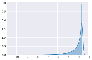
[38]:
sns.distplot(trace.get_sampler_stats('model_logp'))
pass
[39]:
p = trace.get_values('p')
p.shape
[39]:
(8000,)
[40]:
trace['p'].shape
[40]:
(8000,)
Convert to pandas data frame for downstream processing
[41]:
df = pm.trace_to_dataframe(trace)
df.head()
[41]:
| p | |
|---|---|
| 0 | 0.562788 |
| 1 | 0.562788 |
| 2 | 0.476988 |
| 3 | 0.554808 |
| 4 | 0.585853 |
Calculate effective sample size
where \(m\) is the number of chains, \(n\) the number of steps per chain, \(T\) the time when the autocorrelation first becomes negative, and \(\hat{\rho}_t\) the autocorrelation at lag \(t\).
[44]:
pm.effective_n(trace)
[44]:
<xarray.Dataset>
Dimensions:  ()
Data variables:
    p        float64 2.883e+03
Evaluate convergence
Model checking and diagnostics
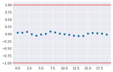
where \(W\) is the within-chain variance and the numeratro is the posterior variance estimate for the pooled traces. Values greater than one indicate that one or more chains have not yet converged.
[45]:
pm.gelman_rubin(trace)
[45]:
<xarray.Dataset>
Dimensions:  ()
Data variables:
    p        float64 1.001
Compares mean and variance of initial with later segments of a trace for a parameter. Should have absolute value less than 1 at convergence.
[46]:
plt.plot(pm.geweke(trace['p'])[:,1], 'o')
plt.axhline(1, c='red')
plt.axhline(-1, c='red')
plt.gca().margins(0.05)
pass
[47]:
pm.summary(trace, varnames=['p'])
[47]:
| mean | sd | hpd_3% | hpd_97% | mcse_mean | mcse_sd | ess_mean | ess_sd | ess_bulk | ess_tail | r_hat | |
|---|---|---|---|---|---|---|---|---|---|---|---|
| p | 0.605 | 0.048 | 0.512 | 0.691 | 0.001 | 0.001 | 2869.0 | 2866.0 | 2883.0 | 4939.0 | 1.0 |
[48]:
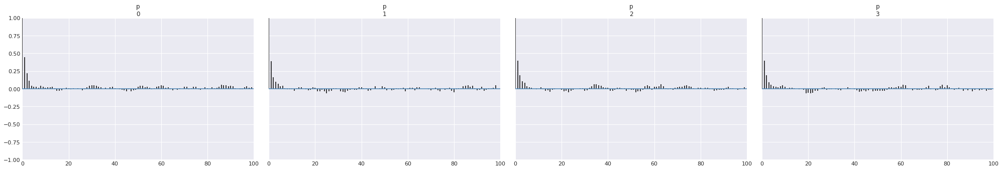
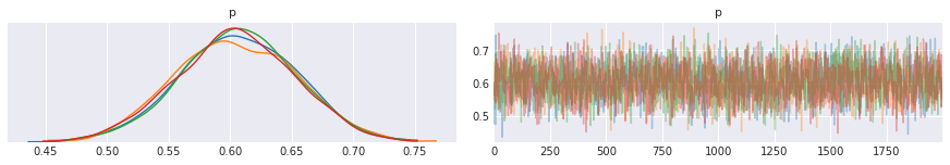
pm.traceplot(trace, varnames=['p'])
pass
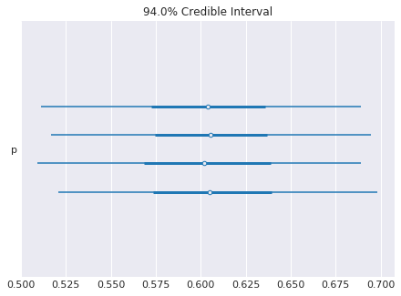
[49]:
pm.forestplot(trace)
pass
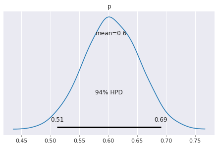
[50]:
pm.plot_posterior(trace)
pass
[51]:
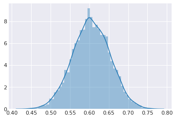
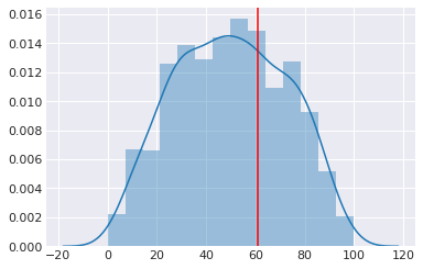
with coin_context:
    ps = pm.sample_prior_predictive(samples=1000)
[52]:
sns.distplot(ps['y'])
plt.axvline(heads, c='red')
pass
[53]:
with coin_context:
    ps = pm.sample_posterior_predictive(trace, samples=1000)
100%|██████████| 1000/1000 [00:00<00:00, 1804.62it/s]
[54]:
sns.distplot(ps['y'])
plt.axvline(heads, c='red')
pass
Saving traces
[55]:
pm.save_trace(trace, 'my_trace', overwrite=True)
[55]:
'my_trace'
You need to re-initialize the model when reloading.
[56]:
with pm.Model() as my_trace:
    p = pm.Beta('p', alpha=2, beta=2)
    y = pm.Binomial('y', n=n, p=p, observed=heads)
    tr = pm.load_trace('my_trace')
[57]:
pm.summary(tr)
[57]:
| mean | sd | hpd_3% | hpd_97% | mcse_mean | mcse_sd | ess_mean | ess_sd | ess_bulk | ess_tail | r_hat | |
|---|---|---|---|---|---|---|---|---|---|---|---|
| p | 0.605 | 0.048 | 0.512 | 0.691 | 0.001 | 0.001 | 2869.0 | 2866.0 | 2883.0 | 4939.0 | 1.0 |
It is probably a good practice to make model reuse convenient
[58]:
def build_model():
    with pm.Model() as m:
        p = pm.Beta('p', alpha=2, beta=2)
        y = pm.Binomial('y', n=n, p=p, observed=heads)
    return m
[59]:
m = build_model()
[60]:
with m:
    tr1 = pm.load_trace('my_trace')
[61]:
pm.summary(tr1)
[61]:
| mean | sd | hpd_3% | hpd_97% | mcse_mean | mcse_sd | ess_mean | ess_sd | ess_bulk | ess_tail | r_hat | |
|---|---|---|---|---|---|---|---|---|---|---|---|
| p | 0.605 | 0.048 | 0.512 | 0.691 | 0.001 | 0.001 | 2869.0 | 2866.0 | 2883.0 | 4939.0 | 1.0 |
Estimating parameters of a normal distribution
[62]:
xs = np.random.normal(5, 2, 20)
Sampling from prior
Just omit the observed= argument.
[63]:
with pm.Model() as prior_context:
    sigma = pm.Gamma('sigma', alpha=2.0, beta=1.0)
    mu = pm.Normal('mu', mu=0, sd=sigma)
    trace = pm.sample(niter, step=pm.Metropolis())
Multiprocess sampling (4 chains in 4 jobs)
CompoundStep
>Metropolis: [mu]
>Metropolis: [sigma]
Sampling 4 chains, 0 divergences: 100%|██████████| 10000/10000 [00:02<00:00, 4894.90draws/s]
The number of effective samples is smaller than 10% for some parameters.
[64]:
pm.traceplot(trace, varnames=['mu', 'sigma'])
pass
Sampling from posterior
[65]:
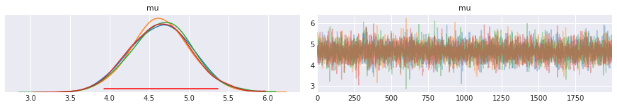
niter = 2000
with pm.Model() as normal_context:
    mu = pm.Normal('mu', mu=0, sd=100)
    sd = pm.HalfCauchy('sd', beta=2)
    y = pm.Normal('y', mu=mu, sd=sd, observed=xs)
    trace = pm.sample(niter)
Auto-assigning NUTS sampler...
Initializing NUTS using jitter+adapt_diag...
Multiprocess sampling (4 chains in 4 jobs)
NUTS: [sd, mu]
Sampling 4 chains, 0 divergences: 100%|██████████| 10000/10000 [00:02<00:00, 3828.57draws/s]
The acceptance probability does not match the target. It is 0.883537546040873, but should be close to 0.8. Try to increase the number of tuning steps.
[66]:
trace.varnames
[66]:
['mu', 'sd_log__', 'sd']
[67]:
hpd = pm.hpd(trace['mu'])
hpd
[67]:
array([3.93067281, 5.36773372])
[68]:
ax = pm.traceplot(trace, varnames=['mu'],)

ymin, ymax = ax[0,0].get_ylim()
y = ymin + 0.05*(ymax-ymin)
ax[0, 0].plot(hpd, [y,y], c='red')
pass
Evaluating goodness-of-fit
WAIC is an approximation to the out-of-sample error and can be used for model comparison. Likelihood is dependent on model complexity and should not be used for model comparisons.
[69]:
with normal_context:
    print(pm.loo(trace))
Computed from 8000 by 20 log-likelihood matrix

       Estimate       SE
IC_loo    78.57     5.65
p_loo      1.70        -
[70]:
with normal_context:
    print(pm.waic(trace))
Computed from 8000 by 20 log-likelihood matrix

        Estimate       SE
IC_waic    78.51     5.61
p_waic      1.67        -

There has been a warning during the calculation. Please check the results.
Comparing models
Use precomputed models for convenience.
[71]:
data1 = az.load_arviz_data("non_centered_eight")
data2 = az.load_arviz_data("centered_eight")
compare_dict = {"non centered": data1, "centered": data2}
az.compare(compare_dict)
[71]:
| rank | waic | p_waic | d_waic | weight | se | dse | warning | waic_scale | |
|---|---|---|---|---|---|---|---|---|---|
| non centered | 0 | 61.292 | 0.800621 | 0 | 0.52814 | 2.5644 | 0 | False | deviance |
| centered | 1 | 61.516 | 0.901656 | 0.223908 | 0.47186 | 2.67176 | 0.155474 | False | deviance |
[72]:
az.compare(compare_dict, ic='LOO')
[72]:
| rank | loo | p_loo | d_loo | weight | se | dse | warning | loo_scale | |
|---|---|---|---|---|---|---|---|---|---|
| non centered | 0 | 61.3746 | 0.841888 | 0 | 0.531189 | 2.58553 | 0 | False | deviance |
| centered | 1 | 61.6207 | 0.954053 | 0.246168 | 0.468811 | 2.69993 | 0.172093 | False | deviance |
Using a custom likelihood
[73]:
def logp(x, μ=0, σ=1):
    """Normal distribtuion."""
    return -0.5*np.log(2*np.pi) - np.log(σ) - (x-μ)**2/(2*σ**2)
[74]:
with pm.Model() as prior_context:
    mu = pm.Normal('mu', mu=0, sd=100)
    sd = pm.HalfCauchy('sd', beta=2)
    y = pm.DensityDist('y', logp, observed=dict(x=xs, μ=mu, σ=sd))
    custom_trace = pm.sample(niter)
Auto-assigning NUTS sampler...
Initializing NUTS using jitter+adapt_diag...
Multiprocess sampling (4 chains in 4 jobs)
NUTS: [sd, mu]
Sampling 4 chains, 0 divergences: 100%|██████████| 10000/10000 [00:02<00:00, 4039.84draws/s]
The acceptance probability does not match the target. It is 0.8804799605408723, but should be close to 0.8. Try to increase the number of tuning steps.
[75]:
pm.trace_to_dataframe(custom_trace).mean()
[75]:
mu    4.634927
sd    1.678608
dtype: float64
Variational methods available
To use a variational method, use pm.fit instead of pm.sample. We’ll see examples of usage in another notebook.
[76]:
print('\n'.join(m for m in dir(pm.variational) if m[0].isupper()))
ADVI
ASVGD
Approximation
Empirical
FullRank
FullRankADVI
Group
ImplicitGradient
Inference
KLqp
MeanField
NFVI
NormalizingFlow
SVGD
Stein
[ ]: