%matplotlib inline

import numpy as np
import pandas as pd
import matplotlib as mpl
import matplotlib.pyplot as plt
import seaborn as sns
import scipy.linalg as la

sns.set_context('notebook', font_scale=1.5)

1. Exact geometric solutions with \(n = m\)

• Find the equation of the line that passes through the points (2,1) and (3,7)

• Find the equation of the circle that passes through the points (1,7), (6,2) and (4,6)

Hint: The equation of a circle can be written as

\[(x - a)^2 + (y - b)^2 = r^2\]

Find the equation of the line that passes through the points (2,1) and (3,7)

Find the equation of the circle that passes through the points (1,7), (6,2) and (4,6)

2. Interpolating polynomials and choice of basis

We have

\(x_i\)	\(y_i\)
0	-5
1	-3
-1	-15
2	39
-2	-9

Find interpolating polynomials using

• Monomial basis \(f_i(x_i) = x^i\) - code this using only simple linear algebra operations (including solve)

• Lagrange basis

  \[l_j(x_j) = \prod_{0 \le m \le k, m \ne j} \frac{x - x_m}{x_j - x_m}\]

The Lagrange interpolation uses the values of \(y\) as the coefficient for the basis polynomials. Do this manually and then using the scipy.interpolate package

x = np.array([0,1,-1,2,-2])
y = np.array([-5, -3, -15, 39, -9])

Monomial basis

Lagrange basis

Using library functions

from scipy.interpolate import lagrange

3. Markov chains

\[\begin{split}P = \pmatrix{ p_{11} & p_{12} & p_{13} \\ p_{21} & p_{22} & p_{33} \\ p_{31} & p_{32} & p_{33} \\ }\end{split}\]

By convention, the \(rows\) of a Markov transition matrix sum to 1, and \(p_{32}\) is the probability that the system will change from state 3 to state 2. Therefore, to see the next state of an initial probability row vector \(v_k\), we need to perform left multiplication

\[v_{k+1}^T = v_{k}^T P\]

If this is confusing, you can work with the matrix \(P^T\) and do right-multiplication with column vectors. In this case, \(p_{32}\) is the probability that the system will change from state 2 to state 3.

Find the stationary vector \(\pi^T = \pi^T P\) for the transition graph shown

• by solving a set of linear equations

• by solving an eigenvector problem

• Check that the resulting vector is invariant with respect to the transition matrix

Brute force check

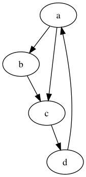
4. Graphs

\(M\) is the adjacency matrix of a directed graph \(G\). Find the vertices that belong to a clique.

\[\begin{split}M = \pmatrix{ 0 & 1 & 0 & 1 & 1 \\ 1 & 0 & 0 & 1 & 0 \\ 1 & 1 & 0 & 1 & 0 \\ 1 & 1 & 0 & 0 & 0 \\ 1 & 0 & 0 & 1 & 0 }\end{split}\]

A clique is defined as a subset of a graph where

1. The subset has at least 3 vertices

2. All pairs of vertices are connected

3. The subset is as large as possible

Because of the symmetry required in condition 2, we only need to consider the graph \(S\) where \(s_{ij} = 1\) if vertcies \(i\) and \(j\) communicate and 0 otherwise. Then the on-zero diagonal entries of \(S^3\) is the set states recurrent in 3 steps. That is, there is a bi-directional path \({s_i \leftrightarrow s_j \leftrightarrow s_k \leftrightarrow s_i}\), which means that the vertices \(\{s_i, s_j, s_k\}\) form a subset of a clique.

M = np.array([
    [0,1,0,1,1],
    [1,0,0,1,1],
    [1,1,0,1,0],
    [1,1,0,0,0],
    [1,0,0,1,0]
])

5. Suppose we wish to solve the problem \(t = Mt + b\) - here the notation is from one type of such problems where \(t\) is the temperature, \(M\) is a matrix for diffusion, and \(b\) represent fixed boundary conditions. Suppose we have a 5 by 5 grid system whose boundary temperatures are fixed. Let \(M\) is a matrix with \(1/4\) for the \(\pm 1\) off-diagonals and 0 elsewhere (i.e. diffusion is approximated by the average temperature of the 4 N, S, E, W neighbors), and \(b\) is the vector \((5,2,3,3,0,1,3,0,1)\) - this assumes the temperatures along the bottom = 0, right edge = 1, top = 2 and left edge = 3. Find the equilibrium temperature at each of the 9 interior points

• by solving a linear equation

• by iteration

Direct solution - not possible for large matrices

Jacobi iteration

6. Iterated affine maps

Define the following mapping in \(\mathbb{R}^2\)

\[\begin{split}T_i: \pmatrix{x \\ y} \to s \pmatrix{\cos \theta & - \sin \theta \\ \sin \theta & \cos \theta} \pmatrix{x \\ y} + \pmatrix{a_i \\ b_i}\end{split}\]

Suppose \(s = 1/3\), \(\theta = 0\), and \(\pmatrix{a_i \\ b_i}\) are

\[\begin{split}\pmatrix{0 \\ 0}, \pmatrix{1/3 \\ 0}, \pmatrix{2/3 \\ 0}, \pmatrix{0 \\ 1/3}, \pmatrix{2/3 \\ 1/3}, \pmatrix{0 \\ 2/3}, \pmatrix{1/3 \\ 2/3}, \pmatrix{2/3 \\ 2/3}\end{split}\]

Generate 1,000 points by first randomly selecting a point in the unit square, then applying at random one of th transformations \(T_i\) to the point. Plot the resulting 1,000 points as a scatter plot on in a square frame.

ab =[
    [0,0],
    [1/3,0],
    [2/3,0],
    [0,1/3],
    [2/3,1/3],
    [0,2/3],
    [1/3,2/3],
    [2/3,2/3]
]

7. The Fibonacci sequence came about from this toy model of rabbit population dynamics

• A baby rabbit matures into an adult in 1 time unit

• An adult gives birth to exactly 1 baby in 1 time unit

• Rabbits are immortal

This gives the well known formula for the number of rabbits over discrete time \(F_{k+2} = F_{k} + F_{k+1}\)

• Express this model as a matrix equation, and calculate the long-term growth rate

Let the population at any time be expreessed as the vector

\[\begin{split}\pmatrix{\text{adult} \\ \text{baby} }\end{split}\]

In the next time step, there will be

• 1 adult from each adult, and one adult from each baby

• 1 baby from each adult

8. Age-structured population growth

Suppose that we observe the following Leslie matrix

\[\begin{split}L = \pmatrix{ 0 & 3 & 2 & 0.5 \\ 0.8 & 0 & 0 & 0 \\ 0 & 0.9 & 0 & 0 \\ 0 & 0 & 0.7 & 0 }\end{split}\]

• Starting with just 1,000 females in age-group 0-15 at time 0 and nobody else, what is the expected population after 90 years?

• Suppose we could alter the fertility in a single age group for this population - can we achieve a steady state non-zero population?

L = np.array([
    [0,3,2,0.5],
    [0.8,0,0,0],
    [0,0.9,0,0],
    [0,0,0.7,0]
])

x0 = np.array([1000,0,0,0]).reshape(-1,1)

Note that the real eigenvalue with real eigenvector is dominant \(\vert L_1 \vert > \vert L_k \vert\).

A theorem says this will be true if you have any two positive consecutive entries in the first row of \(L\).

The growth rate is determined by the dominant real eigenvalue with real eigenvector - in the long term, whether the population will grow, shrink or reach steady state depends on whether this is greater than, less than or equal to 1 respectively.

9.

You are given the following set of data to fit a quadratic polynomial to

x = np.arange(10)
y = np.array([  1.58873597,   7.55101533,  10.71372171,   7.90123225,
                -2.05877605, -12.40257359, -28.64568712, -46.39822281,
                -68.15488905, -97.16032044])

• Find the least squares solution by using the normal equations \(A^T A \hat{x} = A^T y\). (5 points)

x = np.arange(10)
y = np.array([  1.58873597,   7.55101533,  10.71372171,   7.90123225,
                -2.05877605, -12.40257359, -28.64568712, -46.39822281,
                -68.15488905, -97.16032044])

10.

You are given the following data

A = np.array([[1, 8, 0, 7],
       [0, 2, 9, 4],
       [2, 8, 8, 3],
       [4, 8, 6, 1],
       [2, 1, 9, 6],
       [0, 7, 0, 1],
       [4, 0, 2, 4],
       [1, 4, 9, 5],
       [6, 2, 6, 6],
       [9, 9, 6, 3]], dtype='float')

b = np.array([[2],
       [5],
       [0],
       [0],
       [6],
       [7],
       [2],
       [6],
       [7],
       [9]], dtype='float')

• Using SVD directly (not via lstsq), find the least squares solution to \(Ax = b\) (10 points)

• Use SVD to find the best rank 3 approximation of A (10 points)

• Calculate the approximation error in terms of the Frobenius norm (5 points)

A = np.array([[1, 8, 0, 7],
       [0, 2, 9, 4],
       [2, 8, 8, 3],
       [4, 8, 6, 1],
       [2, 1, 9, 6],
       [0, 7, 0, 1],
       [4, 0, 2, 4],
       [1, 4, 9, 5],
       [6, 2, 6, 6],
       [9, 9, 6, 3]], dtype='float')

b = np.array([[2],
       [5],
       [0],
       [0],
       [6],
       [7],
       [2],
       [6],
       [7],
       [9]], dtype='float')

11.

The page rank of a node is given by the equation

and at steady state, we have the page rank vector \(R\)

where \(d\) is the damping factor, \(N\) is the number of nodes, \(1\) is a vector of ones, and

where \(L(p_j)\) is the number of outgoing links from node \(p_j\).

Consider the graph

If \(d = 0.9\) find the page rank of each node

• By solving a linear system

• By eigendecomposition

Note: The Markov matrix constructed as instructed does not follow the usual convention. Here the columns of our Markov matrix are probability vectors, and the page rank is considered to be a column vector of the steady state probabilities.

12.

Recall that a covariance matrix is a matrix whose entries are

1. Find the sample covariance matrix of the 4 features of the iris data set at http://bit.ly/2ow0oJO using basic numpy operations on ndarrasy. Do not use the np.cov or equivalent functions in pandas (except for checking). Remember to scale by \(1/(n-1)\) for the sample covariance. (10 points)

2. Plot the first 2 principal components of the iris data by using eigendecoposition, coloring each data point by the species (10 points)

url = 'http://bit.ly/2ow0oJO'
iris = pd.read_csv(url)
iris.head()

	sepal_length	sepal_width	petal_length	petal_width	species
0	5.1	3.5	1.4	0.2	setosa
1	4.9	3.0	1.4	0.2	setosa
2	4.7	3.2	1.3	0.2	setosa
3	4.6	3.1	1.5	0.2	setosa
4	5.0	3.6	1.4	0.2	setosa