Lab07: Optimization
Brief Honor Code. Do the homework on your own. You may discuss ideas with your classmates, but DO NOT copy the solutions from someone else or the Internet. If stuck, discuss with TA.
Note: The expected figures are provided so you can check your solutions.
1. (20 points)
Find the gradient and Hessian for the following equation
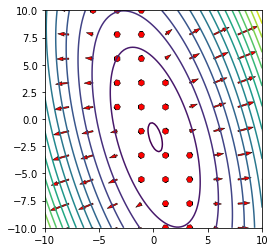
- Plot the contours of this function using
matplotlibin the box \(-5 \le x \le 5\) and \(-5 \le y \le 5\) using a \(100 \times 100\) grid. - Then plot the gradient vectors using the
quiverfunction on top of the contour plot using a \(10 \times 10\) grid. Are the gradients orthogonal to the contours?
Hint: Use numpy.meshgrid, matplotlib.contour and
matplotllib.quiver.
img
In [1]:
2. (30 points)
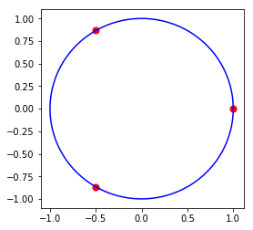
This exercise is about using Newton’s method to find the cube roots of unity - find \(z\) such that \(z^3 = 1\). From the fundamental theorem of algebra, we know there must be exactly 3 complex roots since this is a degree 3 polynomial.
We start with Euler’s equation
Raising \(e^{ix}\) to the \(n\)th power where \(n\) is an integer, we get from Euler’s formula with \(nx\) substituting for \(x\)
Whenever \(nx\) is an integer multiple of \(2\pi\), we have
So
So the cube roots of unity are \(1, e^{2\pi i/3}, e^{4\pi i/3}\).
img
While we can do this analytically, the idea is to use Newton’s method to find these roots, and in the process, discover some rather perplexing behavior of Newton’s method.
Newton’s method for functions of complex variables - stability and basins of attraction. (30 points)
- Write a function with the following function signature
newton(z, f, fprime, max_iter=100, tol=1e-6)wherezis a starting value (a complex number e.g.3 + 4j)fis a function ofzfprimeis the derivative offThe function will run until either max_iter is reached or the absolute value of the Newton step is less than tol. In either case, the function should return the number of iterations taken and the final value ofzas a tuple (i,z).
- Define the function
fandfprimethat will result in Newton’s method finding the cube roots of 1. Find 3 starting points that will give different roots, and print both the start and end points.
Write the following two plotting functions to see some (pretty) aspects of Newton’s algorithm in the complex plane.
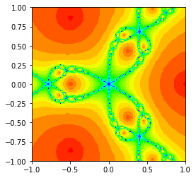
- The first function
plot_newton_iters(f, fprime, n=200, extent=[-1,1,-1,1], cmap='hsv')calculates and stores the number of iterations taken for convergence (or max_iter) for each point in a 2D array. The 2D array limits are given byextent- for example, whenextent = [-1,1,-1,1]the corners of the plot are(-i, -i), (1, -i), (1, i), (-1, i). There arengrid points in both the real and imaginary axes. The argumentcmapspecifies the color map to use - the suggested defaults are fine. Finally plot the image usingplt.imshow- make sure the axis ticks are correctly scaled. Make a plot for the cube roots of 1.
img
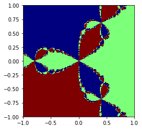
- The second function
plot_newton_basins(f, fprime, n=200, extent=[-1,1,-1,1], cmap='jet')has the same arguments, but this time the grid stores the identity of the root that the starting point converged to. Make a plot for the cube roots of 1 - since there are 3 roots, there should be only 3 colors in the plot.
img
In [1]:
3. (20 points)
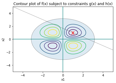
Consider the following function on \(\mathbb{R}^2\):
Find the minimum under the constraint
\[ \begin{align}\begin{aligned}g(x) = x_1^2+x_2^2 \leq 10\\and\end{aligned}\end{align} \]\[ \begin{align}\begin{aligned}h(x) = 2x_1 + 3x_2 = 5\\using ``scipy.optimize.minimize``.\end{aligned}\end{align} \]Plot the function contours using
matplotlib, showing the constraints \(g\) and \(h\) and indicate the constrained minimum with anX.
img
In [1]:
4 (30 points)
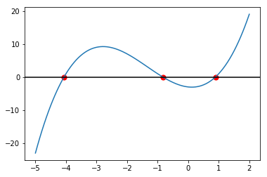
Find solutions to \(x^3 + 4x^2 -3 = x\).
- Write a function to find brackets, assuming roots are always at least 1 unit apart and that the roots lie between -10 and 10
- For each bracket, find the enclosed root using
- a bisection method
- Newton-Raphson (no guarantee to stay within brackets)
- Use the end points of the bracket as starting points for the bisection methods and the midpoint for Newton-Raphson.
- Use the companion matrix and characteristic polynomial to find the solutions
- Plot the function and its roots (marked with a circle) in a window just large enough to contain all roots.
Use a tolerance of 1e-6.
img
In [1]: