In [11]:
%matplotlib inline
In [6]:
import matplotlib.pyplot as plt
import numpy as np
Least squares optimization
Many optimization problems involve minimization of a sum of squared residuals. We will take a look at finding the derivatives for least squares minimization.
In least squares problems, we usually have \(m\) labeled observations \((x_i, y_i)\). We have a model that will predict \(y_i\) given \(x_i\) for some parameters \(\beta\), \(f(x) = X\beta\). We want to minimize the sum (or average) of squared residuals \(r(x_i) = y_i - f(x_i)\). For example, the objective function is usually taken to be
As a concrete example, suppose we want to fit a quadratic function to some observed data. We have
We want to minimize the objective function
Taking derivatives with respect to \(\beta\), we get
Working with matrices
Writing the above system as a matrix, we have \(f(x) = X\beta\), with
and
We want to find the derivative of \(\Vert y - X\beta \Vert^2\), so
Taking derivatives with respect to \(\beta^T\) (we do this because the gradient is traditionally a row vector, and we want it as a column vector here), we get
For example, if we are doing gradient descent, the update equation is
Note that if we set the derivative to zero and solve, we get
and the normal equations
For large \(X\), solving the normal equations can be more expensive than simpler gradient descent. Note that the Levenberg-Marquadt algorithm is often used to optimize least squares problems.
Example
You are given the following set of data to fit a quadratic polynomial to:
x = np.arange(10)
y = np.array([  1.58873597,   7.55101533,  10.71372171,   7.90123225,
                -2.05877605, -12.40257359, -28.64568712, -46.39822281,
                -68.15488905, -97.16032044])
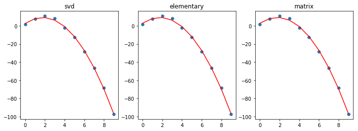
Find the least squares solution using gradient descent.
In [101]:
x = np.arange(10)
y = np.array([  1.58873597,   7.55101533,  10.71372171,   7.90123225,
                -2.05877605, -12.40257359, -28.64568712, -46.39822281,
                -68.15488905, -97.16032044])
In [138]:
def f(x, y, b):
    return (b[0] + b[1]*x + b[2]*x**2 - y)

def res(x, y, b):
    return sum(f(x,y, b)*f(x, y, b))

# Elementary form of gradient
def grad(x, y, b):
    n = len(x)
    return np.array([
            sum(f(x, y, b)),
            sum(x*f(x, y, b)),
            sum(x**2*f(x, y, b))
    ])

# Matrix form of gradient
def grad_m(X, y, b):
    return X.T@X@b- X.T@y
In [139]:
grad(x, y, np.zeros(3))
Out[139]:
array([ 227.0657638 , 1933.9094954 , 15758.14427298])
In [140]:
X = np.c_[np.ones(len(x)), x, x**2]
grad_m(X, y, np.zeros(3))
Out[140]:
array([ 227.0657638 , 1933.9094954 , 15758.14427298])
In [131]:
from scipy.linalg import solve

beta1 = solve(X.T@X, X.T@y)
beta1
Out[131]:
array([ 2.55079998, 7.31478229, -2.04118936])
In [143]:
max_iter = 10000
In [144]:
a = 0.0001 # learning rate
beta2 = np.zeros(3)
for i in range(max_iter):
    beta2 -= a * grad(x, y, beta2)
beta2
Out[144]:
array([ 2.73391723, 7.23152392, -2.03359658])
In [145]:
a = 0.0001 # learning rate
beta3 = np.zeros(3)
for i in range(max_iter):
    beta3 -= a * grad_m(X, y, beta3)
beta3
Out[145]:
array([ 2.73391723, 7.23152392, -2.03359658])
In [146]:
titles = ['svd', 'elementary', 'matrix']

plt.figure(figsize=(12,4))
for i, beta in enumerate([beta1, beta2, beta3], 1):
    plt.subplot(1, 3, i)
    plt.scatter(x, y, s=30)
    plt.plot(x, beta[0] + beta[1]*x + beta[2]*x**2, color='red')
    plt.title(titles[i-1])

Curve fitting and least squares optimization
As shown above, least squares optimization is the technique most
associated with curve fitting. For convenience, scipy.optimize
provides a curve_fit function that uses Levenberg-Marquadt for
minimization.
In [1]:
from scipy.optimize import curve_fit
In [4]:
def logistic4(x, a, b, c, d):
    """The four paramter logistic function is often used to fit dose-response relationships."""
    return ((a-d)/(1.0+((x/c)**b))) + d
In [7]:
nobs = 24
xdata = np.linspace(0.5, 3.5, nobs)
ptrue = [10, 3, 1.5, 12]
ydata = logistic4(xdata, *ptrue) + 0.5*np.random.random(nobs)
In [8]:
popt, pcov = curve_fit(logistic4, xdata, ydata)
In [9]:
perr = yerr=np.sqrt(np.diag(pcov))
print('Param\tTrue\tEstim (+/- 1 SD)')
for p, pt, po, pe  in zip('abcd', ptrue, popt, perr):
    print('%s\t%5.2f\t%5.2f (+/-%5.2f)' % (p, pt, po, pe))
Param   True    Estim (+/- 1 SD)
a       10.00   10.40 (+/- 0.14)
b        3.00    4.20 (+/- 1.16)
c        1.50    1.38 (+/- 0.09)
d       12.00   12.03 (+/- 0.10)
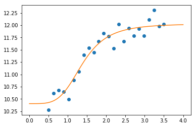
In [13]:
x = np.linspace(0, 4, 100)
y = logistic4(x, *popt)
plt.plot(xdata, ydata, 'o')
plt.plot(x, y)
pass
