Probabilistic Programming
In [1]:
%matplotlib inline
import os
import matplotlib.pyplot as plt
import numpy as np
from scipy import stats
import daft
from IPython.display import Image
import pystan
import seaborn as sns
In [2]:
import warnings
warnings.simplefilter("ignore",category=FutureWarning)
In [3]:
from scipy.optimize import minimize
Domain specific languages (DSL)
A simplified computer language for working in a specific domain. Some examples of DSLs that you are already familiar with include
- regular expressions for working with text
- SQL for working with relational databases
- LaTeX for typesetting documents
Probabilistic programming languages are DSLs for dealing with models
involving random variables and uncertainty. We will introduce the
Stan probabilistic programming languages in this notebook.
Stan and PyStan references
Examples
In general, the problem is set up like this:
We have some observed outcomes \(y\) that we want to model
The model is formulated as a probability distribution with some parameters \(\theta\) to be estimated
We want to estimate the posterior distribution of the model parameters given the data
\[P(\theta \mid y) = \frac{P(y \mid \theta) \, P(\theta)}{\int P(y \mid \theta^*) \, P(\theta^*) \, d\theta^*}\]For formulating a specification using probabilistic programming, it is often useful to think of how we would simulated a draw from the model
Coin bias
We toss a coin \(n\) times, observed the number of times \(y\) it comes up heads, and want to estimate the expected proportion of times \(\theta\) that it comes up heads. An appropriate likelihood is the binomial, and it is convenient to use the \(\beta\) distribution as the prior. In this case, the posterior is also a beta distribution, and there is a simple closed form formula: if the prior is \(\beta(a, b)\) and we observe \(y\) heads and \(n-y\) tails in \(n\) tosses, then the posterior is \(\beta(a+y, a+(n-y)\).
Graphical model
In [4]:
pgm = daft.PGM(shape=[2.5, 3.0], origin=[0, -0.5])

pgm.add_node(daft.Node("alpha", r"$\alpha$", 0.5, 2, fixed=True))
pgm.add_node(daft.Node("beta", r"$\beta$", 1.5, 2, fixed=True))
pgm.add_node(daft.Node("p", r"$p$", 1, 1))
pgm.add_node(daft.Node("n", r"$n$", 2, 0, fixed=True))
pgm.add_node(daft.Node("y", r"$y$", 1, 0, observed=True))

pgm.add_edge("alpha", "p")
pgm.add_edge("beta", "p")
pgm.add_edge("n", "y")
pgm.add_edge("p", "y")

pgm.render()
plt.close()
pgm.figure.savefig("bias.png", dpi=300)
pass
In [5]:
Image("bias.png", width=400)
Out[5]:
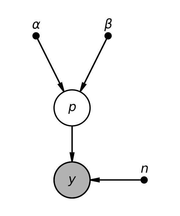
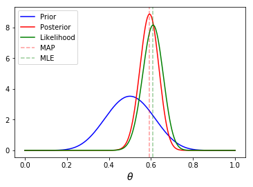
Analytical solution
Illustrating what \(y\), \(\theta\), posterior, likelihood, prior, MLE and MAP refer to.
In [6]:
n = 100
h = 61
p = h/n
rv = stats.binom(n, p)
mu = rv.mean()

a, b = 10, 10
prior = stats.beta(a, b)
post = stats.beta(h+a, n-h+b)
ci = post.interval(0.95)

thetas = np.linspace(0, 1, 200)
plt.plot(thetas, prior.pdf(thetas), label='Prior', c='blue')
plt.plot(thetas, post.pdf(thetas), label='Posterior', c='red')
plt.plot(thetas, n*stats.binom(n, thetas).pmf(h), label='Likelihood', c='green')
plt.axvline((h+a-1)/(n+a+b-2), c='red', linestyle='dashed', alpha=0.4, label='MAP')
plt.axvline(mu/n, c='green', linestyle='dashed', alpha=0.4, label='MLE')
plt.xlabel(r'$\theta$', fontsize=14)
plt.legend(loc='upper left')
plt.show()
pass
Using stan
Coin bias
Data
In [7]:
data = {
    'n': 100,
    'y': 61,
}
Model
In [8]:
code = """
data {
    int<lower=0> n; // number of tosses
    int<lower=0> y; // number of heads
}
transformed data {}
parameters {
    real<lower=0, upper=1> p;
}
transformed parameters {}
model {
    p ~ beta(2, 2);
    y ~ binomial(n, p);
}
generated quantities {}
"""
Compile the C++ model
In [9]:
sm = pystan.StanModel(model_code=code)
INFO:pystan:COMPILING THE C++ CODE FOR MODEL anon_model_7f1947cd2d39ae427cd7b6bb6e6ffd77 NOW.
In [10]:
print(sm.model_cppcode)
// Code generated by Stan version 2.17.1

#include <stan/model/model_header.hpp>

namespace anon_model_7f1947cd2d39ae427cd7b6bb6e6ffd77_namespace {

using std::istream;
using std::string;
using std::stringstream;
using std::vector;
using stan::io::dump;
using stan::math::lgamma;
using stan::model::prob_grad;
using namespace stan::math;

static int current_statement_begin__;

stan::io::program_reader prog_reader__() {
    stan::io::program_reader reader;
    reader.add_event(0, 0, "start", "unknown file name");
    reader.add_event(15, 15, "end", "unknown file name");
    return reader;
}

class anon_model_7f1947cd2d39ae427cd7b6bb6e6ffd77 : public prob_grad {
private:
    int n;
    int y;
public:
    anon_model_7f1947cd2d39ae427cd7b6bb6e6ffd77(stan::io::var_context& context__,
        std::ostream* pstream__ = 0)
        : prob_grad(0) {
        ctor_body(context__, 0, pstream__);
    }

    anon_model_7f1947cd2d39ae427cd7b6bb6e6ffd77(stan::io::var_context& context__,
        unsigned int random_seed__,
        std::ostream* pstream__ = 0)
        : prob_grad(0) {
        ctor_body(context__, random_seed__, pstream__);
    }

    void ctor_body(stan::io::var_context& context__,
                   unsigned int random_seed__,
                   std::ostream* pstream__) {
        typedef double local_scalar_t__;

        boost::ecuyer1988 base_rng__ =
          stan::services::util::create_rng(random_seed__, 0);
        (void) base_rng__;  // suppress unused var warning

        current_statement_begin__ = -1;

        static const char* function__ = "anon_model_7f1947cd2d39ae427cd7b6bb6e6ffd77_namespace::anon_model_7f1947cd2d39ae427cd7b6bb6e6ffd77";
        (void) function__;  // dummy to suppress unused var warning
        size_t pos__;
        (void) pos__;  // dummy to suppress unused var warning
        std::vector<int> vals_i__;
        std::vector<double> vals_r__;
        local_scalar_t__ DUMMY_VAR__(std::numeric_limits<double>::quiet_NaN());
        (void) DUMMY_VAR__;  // suppress unused var warning

        // initialize member variables
        try {
            current_statement_begin__ = 3;
            context__.validate_dims("data initialization", "n", "int", context__.to_vec());
            n = int(0);
            vals_i__ = context__.vals_i("n");
            pos__ = 0;
            n = vals_i__[pos__++];
            current_statement_begin__ = 4;
            context__.validate_dims("data initialization", "y", "int", context__.to_vec());
            y = int(0);
            vals_i__ = context__.vals_i("y");
            pos__ = 0;
            y = vals_i__[pos__++];

            // validate, data variables
            current_statement_begin__ = 3;
            check_greater_or_equal(function__,"n",n,0);
            current_statement_begin__ = 4;
            check_greater_or_equal(function__,"y",y,0);
            // initialize data variables


            // validate transformed data

            // validate, set parameter ranges
            num_params_r__ = 0U;
            param_ranges_i__.clear();
            current_statement_begin__ = 8;
            ++num_params_r__;
        } catch (const std::exception& e) {
            stan::lang::rethrow_located(e, current_statement_begin__, prog_reader__());
            // Next line prevents compiler griping about no return
            throw std::runtime_error("*** IF YOU SEE THIS, PLEASE REPORT A BUG ***");
        }
    }

    ~anon_model_7f1947cd2d39ae427cd7b6bb6e6ffd77() { }


    void transform_inits(const stan::io::var_context& context__,
                         std::vector<int>& params_i__,
                         std::vector<double>& params_r__,
                         std::ostream* pstream__) const {
        stan::io::writer<double> writer__(params_r__,params_i__);
        size_t pos__;
        (void) pos__; // dummy call to supress warning
        std::vector<double> vals_r__;
        std::vector<int> vals_i__;

        if (!(context__.contains_r("p")))
            throw std::runtime_error("variable p missing");
        vals_r__ = context__.vals_r("p");
        pos__ = 0U;
        context__.validate_dims("initialization", "p", "double", context__.to_vec());
        double p(0);
        p = vals_r__[pos__++];
        try {
            writer__.scalar_lub_unconstrain(0,1,p);
        } catch (const std::exception& e) {
            throw std::runtime_error(std::string("Error transforming variable p: ") + e.what());
        }

        params_r__ = writer__.data_r();
        params_i__ = writer__.data_i();
    }

    void transform_inits(const stan::io::var_context& context,
                         Eigen::Matrix<double,Eigen::Dynamic,1>& params_r,
                         std::ostream* pstream__) const {
      std::vector<double> params_r_vec;
      std::vector<int> params_i_vec;
      transform_inits(context, params_i_vec, params_r_vec, pstream__);
      params_r.resize(params_r_vec.size());
      for (int i = 0; i < params_r.size(); ++i)
        params_r(i) = params_r_vec[i];
    }


    template <bool propto__, bool jacobian__, typename T__>
    T__ log_prob(vector<T__>& params_r__,
                 vector<int>& params_i__,
                 std::ostream* pstream__ = 0) const {

        typedef T__ local_scalar_t__;

        local_scalar_t__ DUMMY_VAR__(std::numeric_limits<double>::quiet_NaN());
        (void) DUMMY_VAR__;  // suppress unused var warning

        T__ lp__(0.0);
        stan::math::accumulator<T__> lp_accum__;

        try {
            // model parameters
            stan::io::reader<local_scalar_t__> in__(params_r__,params_i__);

            local_scalar_t__ p;
            (void) p;  // dummy to suppress unused var warning
            if (jacobian__)
                p = in__.scalar_lub_constrain(0,1,lp__);
            else
                p = in__.scalar_lub_constrain(0,1);


            // transformed parameters


            // validate transformed parameters

            const char* function__ = "validate transformed params";
            (void) function__;  // dummy to suppress unused var warning

            // model body

            current_statement_begin__ = 12;
            lp_accum__.add(beta_log<propto__>(p, 2, 2));
            current_statement_begin__ = 13;
            lp_accum__.add(binomial_log<propto__>(y, n, p));

        } catch (const std::exception& e) {
            stan::lang::rethrow_located(e, current_statement_begin__, prog_reader__());
            // Next line prevents compiler griping about no return
            throw std::runtime_error("*** IF YOU SEE THIS, PLEASE REPORT A BUG ***");
        }

        lp_accum__.add(lp__);
        return lp_accum__.sum();

    } // log_prob()

    template <bool propto, bool jacobian, typename T_>
    T_ log_prob(Eigen::Matrix<T_,Eigen::Dynamic,1>& params_r,
               std::ostream* pstream = 0) const {
      std::vector<T_> vec_params_r;
      vec_params_r.reserve(params_r.size());
      for (int i = 0; i < params_r.size(); ++i)
        vec_params_r.push_back(params_r(i));
      std::vector<int> vec_params_i;
      return log_prob<propto,jacobian,T_>(vec_params_r, vec_params_i, pstream);
    }


    void get_param_names(std::vector<std::string>& names__) const {
        names__.resize(0);
        names__.push_back("p");
    }


    void get_dims(std::vector<std::vector<size_t> >& dimss__) const {
        dimss__.resize(0);
        std::vector<size_t> dims__;
        dims__.resize(0);
        dimss__.push_back(dims__);
    }

    template <typename RNG>
    void write_array(RNG& base_rng__,
                     std::vector<double>& params_r__,
                     std::vector<int>& params_i__,
                     std::vector<double>& vars__,
                     bool include_tparams__ = true,
                     bool include_gqs__ = true,
                     std::ostream* pstream__ = 0) const {
        typedef double local_scalar_t__;

        vars__.resize(0);
        stan::io::reader<local_scalar_t__> in__(params_r__,params_i__);
        static const char* function__ = "anon_model_7f1947cd2d39ae427cd7b6bb6e6ffd77_namespace::write_array";
        (void) function__;  // dummy to suppress unused var warning
        // read-transform, write parameters
        double p = in__.scalar_lub_constrain(0,1);
        vars__.push_back(p);

        // declare and define transformed parameters
        double lp__ = 0.0;
        (void) lp__;  // dummy to suppress unused var warning
        stan::math::accumulator<double> lp_accum__;

        local_scalar_t__ DUMMY_VAR__(std::numeric_limits<double>::quiet_NaN());
        (void) DUMMY_VAR__;  // suppress unused var warning

        try {


            // validate transformed parameters

            // write transformed parameters
            if (include_tparams__) {
            }
            if (!include_gqs__) return;
            // declare and define generated quantities


            // validate generated quantities

            // write generated quantities
        } catch (const std::exception& e) {
            stan::lang::rethrow_located(e, current_statement_begin__, prog_reader__());
            // Next line prevents compiler griping about no return
            throw std::runtime_error("*** IF YOU SEE THIS, PLEASE REPORT A BUG ***");
        }
    }

    template <typename RNG>
    void write_array(RNG& base_rng,
                     Eigen::Matrix<double,Eigen::Dynamic,1>& params_r,
                     Eigen::Matrix<double,Eigen::Dynamic,1>& vars,
                     bool include_tparams = true,
                     bool include_gqs = true,
                     std::ostream* pstream = 0) const {
      std::vector<double> params_r_vec(params_r.size());
      for (int i = 0; i < params_r.size(); ++i)
        params_r_vec[i] = params_r(i);
      std::vector<double> vars_vec;
      std::vector<int> params_i_vec;
      write_array(base_rng,params_r_vec,params_i_vec,vars_vec,include_tparams,include_gqs,pstream);
      vars.resize(vars_vec.size());
      for (int i = 0; i < vars.size(); ++i)
        vars(i) = vars_vec[i];
    }

    static std::string model_name() {
        return "anon_model_7f1947cd2d39ae427cd7b6bb6e6ffd77";
    }


    void constrained_param_names(std::vector<std::string>& param_names__,
                                 bool include_tparams__ = true,
                                 bool include_gqs__ = true) const {
        std::stringstream param_name_stream__;
        param_name_stream__.str(std::string());
        param_name_stream__ << "p";
        param_names__.push_back(param_name_stream__.str());

        if (!include_gqs__ && !include_tparams__) return;

        if (include_tparams__) {
        }


        if (!include_gqs__) return;
    }


    void unconstrained_param_names(std::vector<std::string>& param_names__,
                                   bool include_tparams__ = true,
                                   bool include_gqs__ = true) const {
        std::stringstream param_name_stream__;
        param_name_stream__.str(std::string());
        param_name_stream__ << "p";
        param_names__.push_back(param_name_stream__.str());

        if (!include_gqs__ && !include_tparams__) return;

        if (include_tparams__) {
        }


        if (!include_gqs__) return;
    }

}; // model

}

typedef anon_model_7f1947cd2d39ae427cd7b6bb6e6ffd77_namespace::anon_model_7f1947cd2d39ae427cd7b6bb6e6ffd77 stan_model;
MAP
In [11]:
fit_map = sm.optimizing(data=data)
In [12]:
fit_map.keys()
Out[12]:
odict_keys(['p'])
In [13]:
fit_map.get('p')
Out[13]:
array(0.60784305)
In [14]:
fit = sm.sampling(data=data, iter=1000, chains=4)
Summarizing the MCMC fit
In [15]:
print(fit.stansummary())
Inference for Stan model: anon_model_7f1947cd2d39ae427cd7b6bb6e6ffd77.
4 chains, each with iter=1000; warmup=500; thin=1;
post-warmup draws per chain=500, total post-warmup draws=2000.

       mean se_mean     sd   2.5%    25%    50%    75%  97.5%  n_eff   Rhat
p      0.61  1.6e-3   0.05   0.51   0.57   0.61   0.64    0.7    865    1.0
lp__ -70.25    0.03   0.71 -72.29 -70.42 -69.97  -69.8 -69.74    728    1.0

Samples were drawn using NUTS at Wed Mar 21 09:57:17 2018.
For each parameter, n_eff is a crude measure of effective sample size,
and Rhat is the potential scale reduction factor on split chains (at
convergence, Rhat=1).
Interpreting n_eff and Rhat
Effective sample size
where \(m\) is the number of chains, \(n\) the number of steps per chain, \(T\) the time when the autocorrelation first becomes negative, and \(\hat{\rho}_t\) the autocorrelation at lag \(t\).
Gelman-Rubin \(\widehat{R}\)
where \(W\) is the within-chain variance and \(\widehat{V}\) is the posterior variance estimate for the pooled traces. Values greater than one indicate that one or more chains have not yet converged.
Discrad burn-in steps for each chain. The idea is to see if the starting values of each chain come from the same distribution as the stationary state.
- \(W\) is the number of chains \(m \times\) the variacne of each individual chain
- \(B\) is the number of steps \(n \times\) the variance of the chain means
- \(\widehat{V}\) is the weigthed average \((1 - \frac{1}{n})W + \frac{1}{n}B\)
The idea is that \(\widehat{V}\) is an unbiased estimator of \(W\) if the starting values of each chain come from the same distribution as the stationary state. Hence if \(\widehat{R}\) differs significantly from 1, there is probably no convergence and we need more iterations. This is done for each parameter \(\theta\).
\(\widehat{R}\) is a measure of chain convergence
In [16]:
ps = fit.extract(None, permuted=False)
WARNING:root:`dtypes` ignored when `permuted` is False.
In [17]:
fit.model_pars
Out[17]:
['p']
In [18]:
ps.shape
Out[18]:
(500, 4, 2)
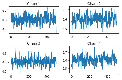
In [19]:
fig, axes = plt.subplots(2,2)
for i, ax in enumerate(axes.ravel()):
    ax.plot(ps[:, i, 0])
    ax.set_title('Chain %d' % (i+1))
plt.tight_layout()
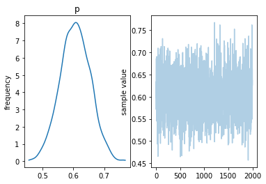
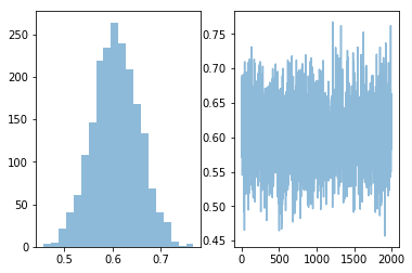
Extracting parameters
In [21]:
params = fit.extract()
In [22]:
p = params['p']
plt.subplot(121)
plt.hist(p, 20, alpha=0.5)
plt.subplot(122)
plt.plot(p, alpha=0.5)
pass
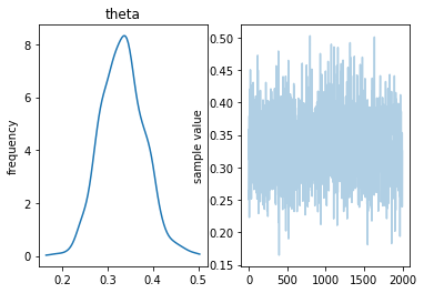
Coin toss as Bernoulli model
In [23]:
%%file bernoulli_model.stan
data {
int<lower=0> N;
int<lower=0,upper=1> y[N];
}
parameters {
real<lower=0,upper=1> theta;
}
model {
theta ~ beta(1,1);
for (n in 1:N)
y[n] ~ bernoulli(theta);
}
Overwriting bernoulli_model.stan
In [24]:
y = np.random.choice([0,1], 100, p=[0.6, 0.4])
data = {
'N': len(y),
'y': y
}
In [25]:
sm = pystan.StanModel('bernoulli_model.stan')
INFO:pystan:COMPILING THE C++ CODE FOR MODEL anon_model_fb711f588d2bebfe1cfbb8d68ae0845e NOW.
In [26]:
fit = sm.sampling(data=data, iter=1000, chains=4)
In [27]:
fit
Out[27]:
Inference for Stan model: anon_model_fb711f588d2bebfe1cfbb8d68ae0845e.
4 chains, each with iter=1000; warmup=500; thin=1;
post-warmup draws per chain=500, total post-warmup draws=2000.
mean se_mean sd 2.5% 25% 50% 75% 97.5% n_eff Rhat
theta 0.33 1.7e-3 0.05 0.24 0.3 0.33 0.36 0.43 756 1.01
lp__ -65.46 0.03 0.8 -67.62 -65.65 -65.17 -64.98 -64.92 956 1.0
Samples were drawn using NUTS at Wed Mar 21 09:58:26 2018.
For each parameter, n_eff is a crude measure of effective sample size,
and Rhat is the potential scale reduction factor on split chains (at
convergence, Rhat=1).
In [28]:
fit.plot()
pass
MAP
In [29]:
opt = sm.optimizing(data)
In [30]:
opt
Out[30]:
OrderedDict([('theta', array(0.33000006))])
The MAP maximizes the log probability of the model.
In [31]:
xi = np.linspace(0, 1, 100)
plt.plot(xi, [fit.log_prob(np.log(x) - np.log(1-x)) for x in xi])
pass
/usr/local/lib/python3.6/site-packages/ipykernel_launcher.py:2: RuntimeWarning: divide by zero encountered in log
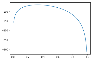
Stan automatically transforms variables so as to work with unconstrained optimization. Knowing this, we can try to replicate the optimization procedure.
In [32]:
p0 = 0.1
x0 = np.log(p0) - np.log(1 - p0)
sol = minimize(fun=lambda x: -fit.log_prob(x), x0=x0)
In [33]:
sol
Out[33]:
fun: 64.92444516607115
 hess_inv: array([[0.04413613]])
      jac: array([-5.7220459e-06])
  message: 'Optimization terminated successfully.'
     nfev: 21
      nit: 6
     njev: 7
   status: 0
  success: True
        x: array([-0.69314706])
In [34]:
np.exp(sol.x)/(1 + np.exp(sol.x))
Out[34]:
array([0.33333336])
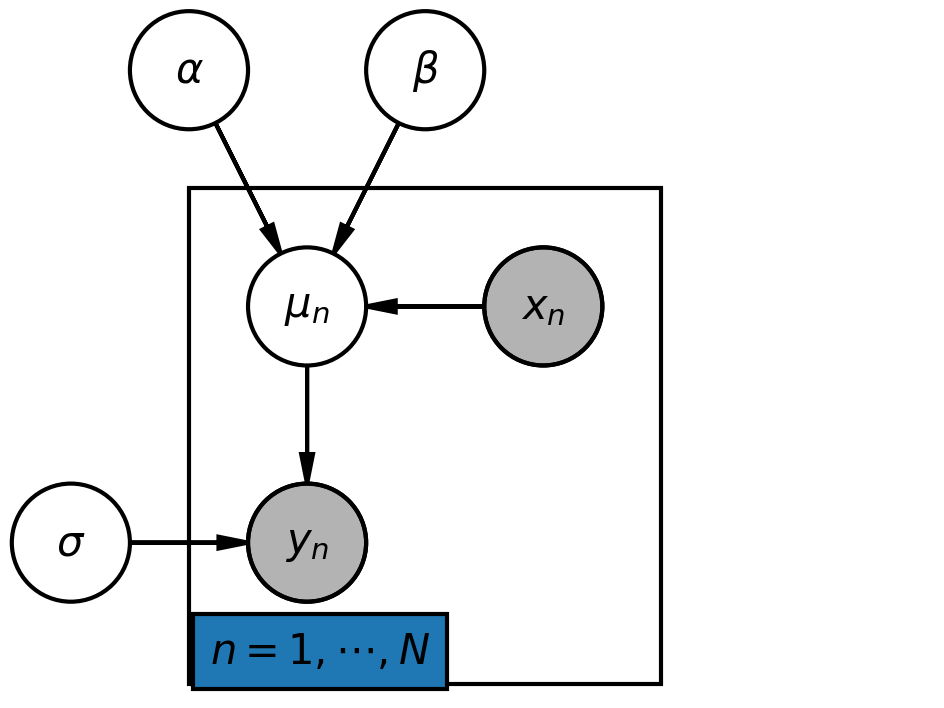
Linear regression
Another simple example of a probabilistic model is linear regression
with \(\epsilon \sim N(0, \sigma^2)\).
We can think of the simulation model as sampling \(y\) from the probability distribution
and the parameter \(\theta = (a, b, \sigma)\) is to be estimated (as posterior probability, MLE or MAP). To complete the model, we need to specify prior distributions for \(a\), \(b\) and \(\sigma\). For example, if the observations \(y\) are standardized to have zero mean and unit standard distribution, we can use
To get a more robust fit that is less sensitive to outliers, we can use a student-T distribution for \(y\)
with an extra parameter \(\nu\) for the degrees of freedom for which we also need to specify a prior.
In [35]:
# Instantiate the PGM.
pgm = daft.PGM(shape=[4.0, 3.0], origin=[-0.3, -0.7])

# Hierarchical parameters.
pgm.add_node(daft.Node("alpha", r"$\alpha$", 0.5, 2))
pgm.add_node(daft.Node("beta", r"$\beta$", 1.5, 2))
pgm.add_node(daft.Node("sigma", r"$\sigma$", 0, 0))

# Deterministic variable.
pgm.add_node(daft.Node("mu", r"$\mu_n$", 1, 1))

# Data.
pgm.add_node(daft.Node("x", r"$x_n$", 2, 1, observed=True))
pgm.add_node(daft.Node("y", r"$y_n$", 1, 0, observed=True))

# Add in the edges.
pgm.add_edge("alpha", "mu")
pgm.add_edge("beta", "mu")
pgm.add_edge("x", "mu")
pgm.add_edge("mu", "y")
pgm.add_edge("sigma", "y")

# And a plate.
pgm.add_plate(daft.Plate([0.5, -0.5, 2, 2], label=r"$n = 1, \cdots, N$",
    shift=-0.1, rect_params={'color': 'white'}))

# Render and save.
pgm.render()
plt.close()
pgm.figure.savefig("lm.png", dpi=300)
In [36]:
Image(filename="lm.png", width=400)
Out[36]:
Linear model
In [38]:
%%file linear.stan

data {
    int<lower=0> N;
    real x[N];
    real y[N];
}

parameters {
    real alpha;
    real beta;
    real<lower=0> sigma; // half-normal distribution
}

transformed parameters {
    real mu[N];
    for (i in 1:N) {
        mu[i] = alpha + beta*x[i];
    }
}

model {
    alpha ~ normal(0, 10);
    beta ~ normal(0, 1);
    sigma ~ normal(0, 1);
    y ~ normal(mu, sigma);
}
Overwriting linear.stan
In [39]:
n = 11
_a = 6
_b = 2
x = np.linspace(0, 1, n)
y = _a + _b*x + np.random.randn(n)

data = {
    'N': n,
    'x': x,
    'y': y
}
Saving and reloading compiled models
Since Stan models take a while to compile, we will define two convenience functions to save and load them. For example, this will allow reuse of the mode in a different session or notebook without recompilation.
In [40]:
import pickle

def save(filename, x):
    with open(filename, 'wb') as f:
        pickle.dump(x, f, protocol=pickle.HIGHEST_PROTOCOL)

def load(filename):
    with open(filename, 'rb') as f:
        return pickle.load(f)
In [41]:
model_name = 'linear'
filename = '%s.pkl' % model_name
if not os.path.exists(filename):
    sm = pystan.StanModel('%s.stan' % model_name)
    save(filename, sm)
else:
    sm = load(filename)
We can inspect the original model from the loaded compiled version.
In [42]:
print(sm.model_code)
data {
    int<lower=0> N;
    real x[N];
    real y[N];
}

parameters {
    real alpha;
    real beta;
    real<lower=0> sigma;
}

transformed parameters {
    real mu[N];
    for (i in 1:N) {
        mu[i] = alpha*x[i] + beta;
    }
}

model {
    alpha ~ normal(0, 10);
    beta ~ normal(0, 1);
    sigma ~ normal(0, 1);
    y ~ normal(mu, sigma);
}
In [43]:
fit = sm.sampling(data)
In [44]:
fit
Out[44]:
Inference for Stan model: anon_model_3e02a2e67db7786f6ac294d214bdf9b6.
4 chains, each with iter=2000; warmup=1000; thin=1;
post-warmup draws per chain=1000, total post-warmup draws=4000.

         mean se_mean     sd   2.5%    25%    50%    75%  97.5%  n_eff   Rhat
alpha    6.33    0.06   1.79    3.2   5.03    6.2   7.51   10.1    945    1.0
beta     3.21    0.04   1.06   1.05   2.47   3.24   3.99   5.15    868    1.0
sigma    1.82    0.02   0.49   0.99   1.46   1.77   2.14   2.85   1027    1.0
mu[0]    3.21    0.04   1.06   1.05   2.47   3.24   3.99   5.15    868    1.0
mu[1]    3.84    0.03   0.92   1.97   3.21   3.87   4.51   5.53    905    1.0
mu[2]    4.48    0.03   0.79   2.87   3.94    4.5   5.05   5.91    987    1.0
mu[3]    5.11    0.02   0.68   3.71   4.66   5.13    5.6   6.33   1174    1.0
mu[4]    5.74    0.02   0.61   4.44   5.35   5.78   6.18   6.79   1633    1.0
mu[5]    6.37    0.01   0.58    5.1   6.01   6.42   6.78   7.36   2613    1.0
mu[6]    7.01  9.6e-3   0.61   5.71   6.63   7.04   7.41    8.1   4000    1.0
mu[7]    7.64    0.01   0.69   6.25    7.2   7.66   8.08   8.98   3403    1.0
mu[8]    8.27    0.02   0.79   6.73   7.77   8.26   8.76    9.9   2687    1.0
mu[9]    8.91    0.02   0.93   7.18    8.3   8.86   9.46  10.84   2126    1.0
mu[10]   9.54    0.03   1.07   7.58   8.83   9.47  10.19  11.79   1797    1.0
lp__   -20.08    0.03   1.27 -23.37 -20.61 -19.75 -19.17 -18.62   1439    1.0

Samples were drawn using NUTS at Wed Mar 21 09:58:27 2018.
For each parameter, n_eff is a crude measure of effective sample size,
and Rhat is the potential scale reduction factor on split chains (at
convergence, Rhat=1).
Re-using the model on a new data set
In [45]:
n = 121
_a = 2
_b = 1
x = np.linspace(0, 1, n)
y = _a*x + _b + np.random.randn(n)

data = {
    'N': n,
    'x': x,
    'y': y
}
In [46]:
fit2 = sm.sampling(data)
In [47]:
print(fit2.stansummary(pars=['alpha', 'beta', 'sigma']))
Inference for Stan model: anon_model_3e02a2e67db7786f6ac294d214bdf9b6.
4 chains, each with iter=2000; warmup=1000; thin=1;
post-warmup draws per chain=1000, total post-warmup draws=4000.

        mean se_mean     sd   2.5%    25%    50%    75%  97.5%  n_eff   Rhat
alpha   1.18  7.7e-3    0.3   0.59   0.98   1.18   1.38   1.77   1501    1.0
beta    1.29  4.2e-3   0.17   0.96   1.17   1.29   1.41   1.63   1661    1.0
sigma   0.98  1.4e-3   0.06   0.87   0.94   0.98   1.02    1.1   1870    1.0

Samples were drawn using NUTS at Wed Mar 21 09:58:28 2018.
For each parameter, n_eff is a crude measure of effective sample size,
and Rhat is the potential scale reduction factor on split chains (at
convergence, Rhat=1).
Hierarchical models
Gelman’s book has an example where the dose of a drug may be affected to the number of rat deaths in an experiment.
| Dose (log g/ml) | # Rats | # Deaths |
|---|---|---|
| -0.896 | 5 | 0 |
| -0.296 | 5 | 1 |
| -0.053 | 5 | 3 |
| 0.727 | 5 | 5 |
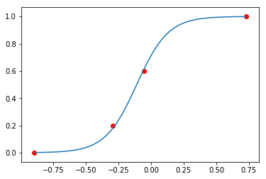
We will model the number of deaths as a random sample from a binomial distribution, where \(n\) is the number of rats and \(p\) the probability of a rat dying. We are given \(n = 5\), but we believe that \(p\) may be related to the drug dose \(x\). As \(x\) increases the number of rats dying seems to increase, and since \(p\) is a probability, we use the following model:
where we set vague priors for \(\alpha\) and \(\beta\), the parameters for the logistic model.
Exercise: Create the plate diagram for this model using daft.
Hierarchical model in Stan
In [48]:
data = dict(
    N = 4,
    x = [-0.896, -0.296, -0.053, 0.727],
    y = [0, 1, 3, 5],
    n = [5, 5, 5, 5],
)
In [49]:
%%file dose.stan

data {
    int<lower=0> N;
    int<lower=0> n[N];
    real x[N];
    int<lower=0> y[N];
}

parameters {
    real alpha;
    real beta;
}

transformed parameters {
    real <lower=0, upper=1> p[N];
    for (i in 1:N) {
        p[i] = inv_logit(alpha + beta*x[i]);
    }
}

model {
    alpha ~ normal(0, 5);
    beta ~ normal(0, 10);
    for (i in 1:N) {
        y ~ binomial(n, p);
    }
}
Overwriting dose.stan
In [50]:
model_name = 'dose'
filename = '%s.pkl' % model_name
if not os.path.exists(filename):
    sm = pystan.StanModel('%s.stan' % model_name)
    save(filename, sm)
else:
    sm = load(filename)
INFO:pystan:COMPILING THE C++ CODE FOR MODEL anon_model_40004ac135c74450331b836ef8235826 NOW.
In [51]:
fit = sm.sampling(data=data)
fit
Out[51]:
Inference for Stan model: anon_model_40004ac135c74450331b836ef8235826.
4 chains, each with iter=2000; warmup=1000; thin=1;
post-warmup draws per chain=1000, total post-warmup draws=4000.

        mean se_mean     sd   2.5%    25%    50%    75%  97.5%  n_eff   Rhat
alpha   0.91    0.02   0.51  -0.01   0.56    0.9   1.25    2.0   1082    1.0
beta    8.29    0.07   2.32   4.49   6.58   8.04   9.76  13.32   1053    1.0
p[0]  4.6e-3  1.8e-4 7.6e-3 2.9e-5 4.9e-4 1.8e-3 5.4e-3   0.03   1889    1.0
p[1]    0.19  1.3e-3   0.07   0.07   0.14   0.18   0.23   0.34   3090    1.0
p[2]    0.61  2.8e-3    0.1   0.42   0.54   0.61   0.68    0.8   1290    1.0
p[3]     1.0  2.6e-4 9.5e-3   0.97    1.0    1.0    1.0    1.0   1321    1.0
lp__  -24.89    0.03    1.0 -27.51 -25.31 -24.59 -24.16 -23.88   1251    1.0

Samples were drawn using NUTS at Wed Mar 21 09:59:36 2018.
For each parameter, n_eff is a crude measure of effective sample size,
and Rhat is the potential scale reduction factor on split chains (at
convergence, Rhat=1).
In [52]:
alpha, beta, *probs = fit.get_posterior_mean()
a = alpha.mean()
b = beta.mean()
Logistic function
In [53]:
def logistic(a, b, x):
    """Logistic function."""
    return np.exp(a + b*x)/(1 + np.exp(a + b*x))
In [54]:
xi =  np.linspace(min(data['x']), max(data['x']), 100)
plt.plot(xi, logistic(a, b, xi))
plt.scatter(data['x'], [y_/n_ for (y_, n_) in zip(data['y'], data['n'])], c='red')
pass
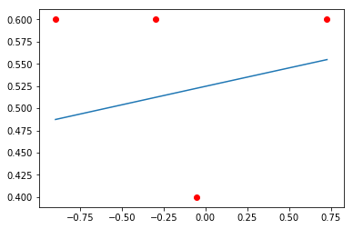
Sampling from prior
In [55]:
%%file dose_prior.stan

data {
    int<lower=0> N;
    int<lower=0> n[N];
    real x[N];
}

parameters {
    real alpha;
    real beta;
}

transformed parameters {
    real <lower=0, upper=1> p[N];
    for (i in 1:N) {
        p[i] = inv_logit(alpha + beta*x[i]);
    }
}

model {
    alpha ~ normal(0, 5);
    beta ~ normal(0, 10);
}
Overwriting dose_prior.stan
In [56]:
sm = pystan.StanModel('dose_prior.stan')
INFO:pystan:COMPILING THE C++ CODE FOR MODEL anon_model_19656edfaafe00f17bef18a5ebf7150a NOW.
In [57]:
fit_prior = sm.sampling(data=data)
In [58]:
alpha, beta, *probs, lp = fit_prior.get_posterior_mean()
a = alpha.mean()
b = beta.mean()
p = [prob.mean() for prob in probs]
In [59]:
p
Out[59]:
[0.49204373896207554,
 0.5049607712489612,
 0.5091310988390625,
 0.5087831209942868]
In [60]:
y = np.random.binomial(5, p)
In [61]:
y
Out[61]:
array([3, 3, 2, 3])
In [62]:
xi =  np.linspace(min(data['x']), max(data['x']), 100)
plt.plot(xi, logistic(a, b, xi))
plt.scatter(data['x'], [y_/n_ for (y_, n_) in zip(y, data['n'])], c='red')
pass
Sampling from posterior
In [63]:
%%file dose_post.stan

data {
    int<lower=0> N;
    int<lower=0> n[N];
    real x[N];
    int<lower=0> y[N];
}

parameters {
    real alpha;
    real beta;
}

transformed parameters {
    real <lower=0, upper=1> p[N];
    for (i in 1:N) {
        p[i] = inv_logit(alpha + beta*x[i]);
    }
}

model {
    alpha ~ normal(0, 5);
    beta ~ normal(0, 10);
    for (i in 1:N) {
        y ~ binomial(n, p);
    }
}

generated quantities {
    int<lower=0> yp[N];
    for (i in 1:N) {
        yp[i] = binomial_rng(n[i], p[i]);
    }
}
Overwriting dose_post.stan
In [64]:
sm = pystan.StanModel('dose_post.stan')
INFO:pystan:COMPILING THE C++ CODE FOR MODEL anon_model_dc9e5eb156c324b98343f4bde238f913 NOW.
In [65]:
fit_post = sm.sampling(data=data)
In [66]:
yp = fit_post.extract('yp')['yp']
In [67]:
yp.shape
Out[67]:
(4000, 4)
In [68]:
np.c_[data['x'], yp.T[:, :6]]
Out[68]:
array([[-0.896,  0.   ,  0.   ,  0.   ,  0.   ,  0.   ,  0.   ],
       [-0.296,  0.   ,  3.   ,  1.   ,  1.   ,  2.   ,  2.   ],
       [-0.053,  3.   ,  5.   ,  1.   ,  3.   ,  4.   ,  4.   ],
       [ 0.727,  5.   ,  5.   ,  5.   ,  5.   ,  5.   ,  5.   ]])