Spark DataFrames

Use Spakr DataFrames rather than RDDs whenever possible. In general, Spark DataFrames are more performant, and the performance is consistent across differnet languagge APIs. Unlike RDDs which are executed on the fly, Spakr DataFrames are compiled using the Catalyst optimiser and an optimal execution path executed by the engine. Since all langugaes compile to the same execution code, there is no difference across languages (unless you use user-defined funcitons UDF).

Start spark

%%spark

Starting Spark application

ID	YARN Application ID	Kind	State	Spark UI	Driver log	Current session?
150	application_1522938745830_0107	pyspark	idle	Link	Link	✔

SparkSession available as 'spark'.

spark.version

u'2.2.0.2.6.3.0-235'

Import native spark functions

import pyspark.sql.functions as F

Import variables to specify schema

from pyspark.sql.types import StructType, StructField, StringType, IntegerType

RDDs and DataFrames

data = [('ann', 'spring', 'math', 98),
        ('ann', 'fall', 'bio', 50),
        ('bob', 'spring', 'stats', 100),
        ('bob', 'fall', 'stats', 92),
        ('bob', 'summer', 'stats', 100),
        ('charles', 'spring', 'stats', 88),
        ('charles', 'fall', 'bio', 100)
       ]

rdd = sc.parallelize(data)

rdd.take(3)

[('ann', 'spring', 'math', 98), ('ann', 'fall', 'bio', 50), ('bob', 'spring', 'stats', 100)]

df = spark.createDataFrame(rdd, ['name', 'semester', 'subject', 'score'])

df.show()

+-------+--------+-------+-----+
|   name|semester|subject|score|
+-------+--------+-------+-----+
|    ann|  spring|   math|   98|
|    ann|    fall|    bio|   50|
|    bob|  spring|  stats|  100|
|    bob|    fall|  stats|   92|
|    bob|  summer|  stats|  100|
|charles|  spring|  stats|   88|
|charles|    fall|    bio|  100|
+-------+--------+-------+-----+

df.show(3)

+----+--------+-------+-----+
|name|semester|subject|score|
+----+--------+-------+-----+
| ann|  spring|   math|   98|
| ann|    fall|    bio|   50|
| bob|  spring|  stats|  100|
+----+--------+-------+-----+
only showing top 3 rows

df.rdd.take(3)

[Row(name=u'ann', semester=u'spring', subject=u'math', score=98), Row(name=u'ann', semester=u'fall', subject=u'bio', score=50), Row(name=u'bob', semester=u'spring', subject=u'stats', score=100)]

df.describe()

DataFrame[summary: string, name: string, semester: string, subject: string, score: string]

Converstion to and from pandas

Make sure your data set can fit into memory before converting to pandas.

pdf = df.toPandas()
pdf

      name semester subject  score
0      ann   spring    math     98
1      ann     fall     bio     50
2      bob   spring   stats    100
3      bob     fall   stats     92
4      bob   summer   stats    100
5  charles   spring   stats     88
6  charles     fall     bio    100

spark.createDataFrame(pdf).show()

+-------+--------+-------+-----+
|   name|semester|subject|score|
+-------+--------+-------+-----+
|    ann|  spring|   math|   98|
|    ann|    fall|    bio|   50|
|    bob|  spring|  stats|  100|
|    bob|    fall|  stats|   92|
|    bob|  summer|  stats|  100|
|charles|  spring|  stats|   88|
|charles|    fall|    bio|  100|
+-------+--------+-------+-----+

Schemas

df.printSchema()

root
 |-- name: string (nullable = true)
 |-- semester: string (nullable = true)
 |-- subject: string (nullable = true)
 |-- score: long (nullable = true)

Data manipulation

Selecting columns

df.select(['name', 'subject', 'score']).show()

+-------+-------+-----+
|   name|subject|score|
+-------+-------+-----+
|    ann|   math|   98|
|    ann|    bio|   50|
|    bob|  stats|  100|
|    bob|  stats|   92|
|    bob|  stats|  100|
|charles|  stats|   88|
|charles|    bio|  100|
+-------+-------+-----+

Filtering rows

df.filter(df['score'] > 90).show()

+-------+--------+-------+-----+
|   name|semester|subject|score|
+-------+--------+-------+-----+
|    ann|  spring|   math|   98|
|    bob|  spring|  stats|  100|
|    bob|    fall|  stats|   92|
|    bob|  summer|  stats|  100|
|charles|    fall|    bio|  100|
+-------+--------+-------+-----+

Mutating values

Using select

df.select(df['name'], df['semester'], df['subject'], df['score'],
          (df['score'] - 10).alias('adj_score')).show()

+-------+--------+-------+-----+---------+
|   name|semester|subject|score|adj_score|
+-------+--------+-------+-----+---------+
|    ann|  spring|   math|   98|       88|
|    ann|    fall|    bio|   50|       40|
|    bob|  spring|  stats|  100|       90|
|    bob|    fall|  stats|   92|       82|
|    bob|  summer|  stats|  100|       90|
|charles|  spring|  stats|   88|       78|
|charles|    fall|    bio|  100|       90|
+-------+--------+-------+-----+---------+

Using withColumn

df.withColumn('sqrt_socre', df['score']/2).show()

+-------+--------+-------+-----+----------+
|   name|semester|subject|score|sqrt_socre|
+-------+--------+-------+-----+----------+
|    ann|  spring|   math|   98|      49.0|
|    ann|    fall|    bio|   50|      25.0|
|    bob|  spring|  stats|  100|      50.0|
|    bob|    fall|  stats|   92|      46.0|
|    bob|  summer|  stats|  100|      50.0|
|charles|  spring|  stats|   88|      44.0|
|charles|    fall|    bio|  100|      50.0|
+-------+--------+-------+-----+----------+

Sorting

df.sort(df['score']).show()

+-------+--------+-------+-----+
|   name|semester|subject|score|
+-------+--------+-------+-----+
|    ann|    fall|    bio|   50|
|charles|  spring|  stats|   88|
|    bob|    fall|  stats|   92|
|    ann|  spring|   math|   98|
|    bob|  summer|  stats|  100|
|charles|    fall|    bio|  100|
|    bob|  spring|  stats|  100|
+-------+--------+-------+-----+

df.sort(df['score'].desc()).show()

+-------+--------+-------+-----+
|   name|semester|subject|score|
+-------+--------+-------+-----+
|    bob|  summer|  stats|  100|
|    bob|  spring|  stats|  100|
|charles|    fall|    bio|  100|
|    ann|  spring|   math|   98|
|    bob|    fall|  stats|   92|
|charles|  spring|  stats|   88|
|    ann|    fall|    bio|   50|
+-------+--------+-------+-----+

Alternative syntax

df.sort(df.score.desc()).show()

+-------+--------+-------+-----+
|   name|semester|subject|score|
+-------+--------+-------+-----+
|    bob|  spring|  stats|  100|
|charles|    fall|    bio|  100|
|    bob|  summer|  stats|  100|
|    ann|  spring|   math|   98|
|    bob|    fall|  stats|   92|
|charles|  spring|  stats|   88|
|    ann|    fall|    bio|   50|
+-------+--------+-------+-----+

Summarizing

df.agg(
    {'score': 'mean'}
).show()

+-----------------+
|       avg(score)|
+-----------------+
|89.71428571428571|
+-----------------+

df.agg(
    F.mean(df.score).alias('avg'),
    F.min(df.score).alias('min'),
    F.max(df.score).alias('max')
).show()

+-----------------+---+---+
|              avg|min|max|
+-----------------+---+---+
|89.71428571428571| 50|100|
+-----------------+---+---+

Split-Apply-Combine

df.groupby('name').agg({'score': 'mean', 'subject': 'count'}).show()

+-------+-----------------+--------------+
|   name|       avg(score)|count(subject)|
+-------+-----------------+--------------+
|charles|             94.0|             2|
|    ann|             74.0|             2|
|    bob|97.33333333333333|             3|
+-------+-----------------+--------------+

Join

meta = [('ann', 'female', 23),
        ('bob', 'male', 19),
        ('charles', 'male', 22),
        ('daivd', 'male', 23)
       ]

schema = StructType([
    StructField('name', StringType(), True),
    StructField('sex', StringType(), True),
    StructField('age', IntegerType(), True)
])

df_meta = spark.createDataFrame(meta, schema)

df_meta.printSchema()

root
 |-- name: string (nullable = true)
 |-- sex: string (nullable = true)
 |-- age: integer (nullable = true)

df_meta.show()

+-------+------+---+
|   name|   sex|age|
+-------+------+---+
|    ann|female| 23|
|    bob|  male| 19|
|charles|  male| 22|
|  daivd|  male| 23|
+-------+------+---+

df.join(df_meta, on='name', how='inner').show()

+-------+--------+-------+-----+------+---+
|   name|semester|subject|score|   sex|age|
+-------+--------+-------+-----+------+---+
|charles|  spring|  stats|   88|  male| 22|
|charles|    fall|    bio|  100|  male| 22|
|    ann|  spring|   math|   98|female| 23|
|    ann|    fall|    bio|   50|female| 23|
|    bob|  spring|  stats|  100|  male| 19|
|    bob|    fall|  stats|   92|  male| 19|
|    bob|  summer|  stats|  100|  male| 19|
+-------+--------+-------+-----+------+---+

df_full = df.join(df_meta, on='name', how='rightouter')
df_full.drop()

DataFrame[name: string, semester: string, subject: string, score: bigint, sex: string, age: int]

df_full.groupby('sex').mean().show()

+------+----------+------------------+
|   sex|avg(score)|          avg(age)|
+------+----------+------------------+
|female|      74.0|              23.0|
|  male|      96.0|20.666666666666668|
+------+----------+------------------+

df_full.groupby('sex').pivot('subject').agg(F.mean('age')).show()

+------+----+----+----+-----+
|   sex|null| bio|math|stats|
+------+----+----+----+-----+
|female|null|23.0|23.0| null|
|  male|23.0|22.0|null|19.75|
+------+----+----+----+-----+

(
    df_full.
    dropna().
    groupby('sex').
    pivot('subject').
    agg(F.mean('age')).
    show()
)

+------+----+----+-----+
|   sex| bio|math|stats|
+------+----+----+-----+
|female|23.0|23.0| null|
|  male|22.0|null|19.75|
+------+----+----+-----+

Using SQL

df_full.createOrReplaceTempView('table')

Select columns

spark.sql('select name, age from table').show()

+-------+---+
|   name|age|
+-------+---+
|charles| 22|
|charles| 22|
|    ann| 23|
|    ann| 23|
|  daivd| 23|
|    bob| 19|
|    bob| 19|
|    bob| 19|
+-------+---+

Filter rows

spark.sql('select name, age from table where age > 20').show()

+-------+---+
|   name|age|
+-------+---+
|charles| 22|
|charles| 22|
|    ann| 23|
|    ann| 23|
|  daivd| 23|
+-------+---+

Mutate

spark.sql('select name, age + 2 as adj_age from table').show()

+-------+-------+
|   name|adj_age|
+-------+-------+
|charles|     24|
|charles|     24|
|    ann|     25|
|    ann|     25|
|  daivd|     25|
|    bob|     21|
|    bob|     21|
|    bob|     21|
+-------+-------+

Sort

spark.sql('select name, age from table order by age desc').show()

+-------+---+
|   name|age|
+-------+---+
|  daivd| 23|
|    ann| 23|
|    ann| 23|
|charles| 22|
|charles| 22|
|    bob| 19|
|    bob| 19|
|    bob| 19|
+-------+---+

Summary

spark.sql('select mean(age) from table').show()

+--------+
|avg(age)|
+--------+
|   21.25|
+--------+

Split-apply-combine

q = '''
select sex, mean(score), min(age)
from table
group by sex
'''

spark.sql(q).show()

+------+----------+--------+
|   sex|avg(score)|min(age)|
+------+----------+--------+
|female|      74.0|      23|
|  male|      96.0|      19|
+------+----------+--------+

Using SQL magic

%%sql

select sex, mean(score), min(age)
from table
group by sex

Capture output locally (i.e. not sent to livy and cluster)

%%sql -q -o df1

select sex, score, age from table

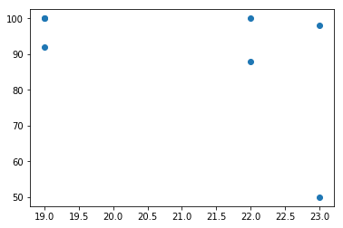
%%local

%matplotlib inline
import matplotlib.pyplot as plt

plt.scatter(x='age', y='score', data=df1)
plt.show()

User Definted Functions (UDF) verus pyspark.sql.functions

Version 1: Using a User Defined Funciton (UDF)

Note: Using a Python UDF is not efficient.

@F.udf
def score_to_grade(g):
    if g > 90:
        return 'A'
    elif g > 80:
        return 'B'
    else:
        return 'C'

df.withColumn('grade', score_to_grade(df['score'])).show()

+-------+--------+-------+-----+-----+
|   name|semester|subject|score|grade|
+-------+--------+-------+-----+-----+
|    ann|  spring|   math|   98|    A|
|    ann|    fall|    bio|   50|    C|
|    bob|  spring|  stats|  100|    A|
|    bob|    fall|  stats|   92|    A|
|    bob|  summer|  stats|  100|    A|
|charles|  spring|  stats|   88|    B|
|charles|    fall|    bio|  100|    A|
+-------+--------+-------+-----+-----+

Version 2: Using built-in fucntions.

See list of functions available.

More performant version

score_to_grade_fast = (
    F.
    when(F.col('score') > 90, 'A').
    when(F.col('score') > 80, 'B').
    otherwise('C')
)

df.withColumn('grade_fast', score_to_grade_fast).show()

+-------+--------+-------+-----+----------+
|   name|semester|subject|score|grade_fast|
+-------+--------+-------+-----+----------+
|    ann|  spring|   math|   98|         A|
|    ann|    fall|    bio|   50|         C|
|    bob|  spring|  stats|  100|         A|
|    bob|    fall|  stats|   92|         A|
|    bob|  summer|  stats|  100|         A|
|charles|  spring|  stats|   88|         B|
|charles|    fall|    bio|  100|         A|
+-------+--------+-------+-----+----------+

Vectorized UDFs

The current version of pyspark 2.3 has support for vectorized UDFs, which can make Python functions using numpy or pandas functionality much faster. Unfortunately, the Docker version of pyspark 2.2 does not support vectorized UDFs.

If you have access to pysark 2.3 see Introducing Pandas UDF for PySpark: How to run your native Python code with PySpark, fast and the linked benchmarking notebook.

I/O options

CSV

df_full.write.mode('overwrite').option('header', 'true').csv('foo.csv')

foo = spark.read.option('header', 'true').csv('foo.csv')

foo.show()

+-------+--------+-------+-----+------+---+
|   name|semester|subject|score|   sex|age|
+-------+--------+-------+-----+------+---+
|    bob|  spring|  stats|  100|  male| 19|
|    bob|    fall|  stats|   92|  male| 19|
|    bob|  summer|  stats|  100|  male| 19|
|charles|  spring|  stats|   88|  male| 22|
|charles|    fall|    bio|  100|  male| 22|
|    ann|  spring|   math|   98|female| 23|
|    ann|    fall|    bio|   50|female| 23|
|  daivd|    null|   null| null|  male| 23|
+-------+--------+-------+-----+------+---+

JSON

df_full.write.mode('overwrite').json('foo.json')

foo = spark.read.json('foo.json')

foo.show()

+---+-------+-----+--------+------+-------+
|age|   name|score|semester|   sex|subject|
+---+-------+-----+--------+------+-------+
| 19|    bob|  100|  spring|  male|  stats|
| 19|    bob|   92|    fall|  male|  stats|
| 19|    bob|  100|  summer|  male|  stats|
| 22|charles|   88|  spring|  male|  stats|
| 22|charles|  100|    fall|  male|    bio|
| 23|    ann|   98|  spring|female|   math|
| 23|    ann|   50|    fall|female|    bio|
| 23|  daivd| null|    null|  male|   null|
+---+-------+-----+--------+------+-------+

Parquet

This is an efficient columnar store.

df_full.write.mode('overwrite').parquet('foo.parquet')

foo = spark.read.parquet('foo.parquet')

foo.show()

+-------+--------+-------+-----+------+---+
|   name|semester|subject|score|   sex|age|
+-------+--------+-------+-----+------+---+
|    bob|  spring|  stats|  100|  male| 19|
|    bob|    fall|  stats|   92|  male| 19|
|    bob|  summer|  stats|  100|  male| 19|
|charles|  spring|  stats|   88|  male| 22|
|charles|    fall|    bio|  100|  male| 22|
|    ann|  spring|   math|   98|female| 23|
|    ann|    fall|    bio|   50|female| 23|
|  daivd|    null|   null| null|  male| 23|
+-------+--------+-------+-----+------+---+

Random numbers

foo.withColumn('uniform', F.rand(seed=123)).show()

+-------+--------+-------+-----+------+---+-------------------+
|   name|semester|subject|score|   sex|age|            uniform|
+-------+--------+-------+-----+------+---+-------------------+
|    bob|  spring|  stats|  100|  male| 19| 0.5029534413816527|
|    bob|    fall|  stats|   92|  male| 19| 0.9867496419260051|
|    bob|  summer|  stats|  100|  male| 19| 0.8209632961670508|
|charles|  spring|  stats|   88|  male| 22|  0.839067819363327|
|charles|    fall|    bio|  100|  male| 22| 0.3737326850860542|
|    ann|  spring|   math|   98|female| 23|0.45650488329285255|
|    ann|    fall|    bio|   50|female| 23| 0.1729393778824495|
|  daivd|    null|   null| null|  male| 23| 0.5760115975887162|
+-------+--------+-------+-----+------+---+-------------------+

foo.withColumn('normal', F.randn(seed=123)).show()

+-------+--------+-------+-----+------+---+--------------------+
|   name|semester|subject|score|   sex|age|              normal|
+-------+--------+-------+-----+------+---+--------------------+
|    bob|  spring|  stats|  100|  male| 19|0.001988081602007817|
|    bob|    fall|  stats|   92|  male| 19| 0.32765099517752727|
|    bob|  summer|  stats|  100|  male| 19| 0.35989602440312274|
|charles|  spring|  stats|   88|  male| 22|  0.3801966195174709|
|charles|    fall|    bio|  100|  male| 22| -2.1726586720908876|
|    ann|  spring|   math|   98|female| 23| -0.7484125450184252|
|    ann|    fall|    bio|   50|female| 23|  -1.229237021920563|
|  daivd|    null|   null| null|  male| 23|  0.2856848655347919|
+-------+--------+-------+-----+------+---+--------------------+

Indexing with row numbers

Note that monotonically_increasing_id works over partitions, so while numbers are guaranteed to be unique and increasing, they may not be consecutive.

foo.withColumn('index', F.monotonically_increasing_id()).show()

+-------+--------+-------+-----+------+---+-----+
|   name|semester|subject|score|   sex|age|index|
+-------+--------+-------+-----+------+---+-----+
|    bob|  spring|  stats|  100|  male| 19|    0|
|    bob|    fall|  stats|   92|  male| 19|    1|
|    bob|  summer|  stats|  100|  male| 19|    2|
|charles|  spring|  stats|   88|  male| 22|    3|
|charles|    fall|    bio|  100|  male| 22|    4|
|    ann|  spring|   math|   98|female| 23|    5|
|    ann|    fall|    bio|   50|female| 23|    6|
|  daivd|    null|   null| null|  male| 23|    7|
+-------+--------+-------+-----+------+---+-----+

Example: Word counting in a DataFrame

There are 2 text files in the /data/texts directory. We will read both in at once.

hadoop = sc._jvm.org.apache.hadoop

fs = hadoop.fs.FileSystem
conf = hadoop.conf.Configuration()
path = hadoop.fs.Path('/data/texts')

for f in fs.get(conf).listStatus(path):
    print f.getPath()

hdfs://vcm-2167.oit.duke.edu:8020/data/texts/Portrait.txt
hdfs://vcm-2167.oit.duke.edu:8020/data/texts/Ulysses.txt

text = spark.read.text('/data/texts')

text.show(10)

+--------------------+
|               value|
+--------------------+
|                    |
|The Project Guten...|
|                    |
|This eBook is for...|
|no restrictions w...|
|it under the term...|
|eBook or online a...|
|                    |
|                    |
|      Title: Ulysses|
+--------------------+
only showing top 10 rows

Remove blank lines

text = text.filter(text['value'] != '')
text.show(10)

+--------------------+
|               value|
+--------------------+
|The Project Guten...|
|This eBook is for...|
|no restrictions w...|
|it under the term...|
|eBook or online a...|
|      Title: Ulysses|
| Author: James Joyce|
|Release Date: Aug...|
|Last Updated: Aug...|
|   Language: English|
+--------------------+
only showing top 10 rows

Using built-in functions to process a column of strings

Note: This is more efficient than using a Python UDF.

from string import punctuation

def process(col):
    col = F.lower(col)                      # convert to lowercase
    col = F.translate(col, punctuation, '') # remove punctuation
    col = F.trim(col)                       # remove leading and traling blank space
    col = F.split(col, '\s')                # split on blank space
    col = F.explode(col)                    # give each iterable in row its owwn row
    return col

words = text.withColumn('value', process(text.value))
words.show(20)

+---------+
|    value|
+---------+
|      the|
|  project|
|gutenberg|
|    ebook|
|       of|
|  ulysses|
|       by|
|    james|
|    joyce|
|     this|
|    ebook|
|       is|
|      for|
|      the|
|      use|
|       of|
|   anyone|
| anywhere|
|       at|
|       no|
+---------+
only showing top 20 rows

counts = words.groupby('value').count()

counts.cache()

DataFrame[value: string, count: bigint]

counts.show(20)

+-----------+-----+
|      value|count|
+-----------+-----+
|     online|    8|
|      those|  403|
|      still|  272|
|   tripping|    5|
|        art|   66|
|        few|  110|
|       some|  416|
|     waters|   47|
|   tortured|    5|
|     slaver|    1|
|      inner|   21|
|       guts|   14|
|       hope|   79|
|     —billy|    1|
|  squealing|    3|
|     deftly|   10|
|     ceylon|    4|
|ineluctably|    4|
|     filing|    3|
|       foxy|    5|
+-----------+-----+
only showing top 20 rows

counts.sort(counts['count'].desc()).show(20)

+-----+-----+
|value|count|
+-----+-----+
|  the|21063|
|   of|11510|
|  and|10611|
|    a| 8500|
|   to| 7033|
|   in| 6555|
|   he| 5835|
|  his| 5069|
| that| 3537|
|   it| 3204|
|  was| 3192|
| with| 3170|
|    i| 2982|
|   on| 2662|
|  you| 2650|
|  for| 2500|
|  him| 2225|
|  her| 2098|
|   is| 1892|
| said| 1821|
+-----+-----+
only showing top 20 rows

counts.sort(counts['count']).show(20)

+-----------------+-----+
|            value|count|
+-----------------+-----+
|          incited|    1|
|     emancipation|    1|
|        overcloud|    1|
|         differed|    1|
|      fruitlessly|    1|
|          outboro|    1|
|            —duck|    1|
|     stonecutting|    1|
|      lectureroom|    1|
|     rainfragrant|    1|
|           lapide|    1|
|         end—what|    1|
|        shielding|    1|
|           breezy|    1|
|        chemistry|    1|
|        —tarentum|    1|
|           hockey|    1|
|            cable|    1|
|         plashing|    1|
|peacocktwittering|    1|
+-----------------+-----+
only showing top 20 rows

spark.stop()