Random Variables
In [1]:
%matplotlib inline
import itertools as it
import re
import matplotlib.pyplot as plt
import numpy as np
import scipy
from scipy import stats
import toolz as tz
Using numpy.random
Setting seed for reproducibility
In [2]:
np.random.seed(123)
Standard uniform
In [3]:
np.random.rand(3,4)
Out[3]:
array([[0.69646919, 0.28613933, 0.22685145, 0.55131477],
       [0.71946897, 0.42310646, 0.9807642 , 0.68482974],
       [0.4809319 , 0.39211752, 0.34317802, 0.72904971]])
Standard normal
In [4]:
np.random.randn(3, 4)
Out[4]:
array([[-0.67888615, -0.09470897,  1.49138963, -0.638902  ],
       [-0.44398196, -0.43435128,  2.20593008,  2.18678609],
       [ 1.0040539 ,  0.3861864 ,  0.73736858,  1.49073203]])
Parameterized distributions
Parameterized distribution functions typically have one or more of location, scale, shape or other parameters that can be specified.
Continuous distributions
In [5]:
np.random.uniform(low=-1, high=1, size=(3, 4))
Out[5]:
array([[ 0.44488677, -0.35408217, -0.27642269, -0.54347354],
       [-0.41257191,  0.26195225, -0.81579012, -0.13259765],
       [-0.13827447, -0.0126298 , -0.14833942, -0.37547755]])
In [6]:
np.random.normal(loc=100, scale=15, size=(3, 4))
Out[6]:
array([[113.91193648,  97.39546476, 100.04268874, 110.32334067],
       [ 86.80695485, 104.25440986,  87.91950223,  74.08495759],
       [ 94.13650309, 108.60708794, 105.07883576,  99.82254258]])
In [7]:
np.random.standard_t(df=3, size=(3,4))
Out[7]:
array([[ 2.26603603,  0.26443366, -2.62014171,  0.73989909],
       [ 0.52766961,  0.84688526, -0.63048839, -0.92233841],
       [ 1.15114019,  0.67780629,  0.82852178,  0.30139753]])
In [8]:
np.random.beta(a=0.5, b=0.5, size=(10,))
Out[8]:
array([0.9853416 , 0.36941327, 0.17888099, 0.42376794, 0.12553194,
       0.32966061, 0.37205691, 0.39564619, 0.19150945, 0.83135736])
Discrete distributions
In [9]:
np.random.poisson(lam=10, size=(10,))
Out[9]:
array([ 8, 8, 11, 15, 8, 7, 13, 12, 9, 9])
In [10]:
np.random.binomial(n=10, p=0.6, size=(10,))
Out[10]:
array([8, 7, 4, 6, 6, 5, 5, 8, 5, 4])
In [11]:
np.random.negative_binomial(n=10, p=0.6, size=(10,))
Out[11]:
array([10, 8, 3, 0, 6, 6, 4, 6, 3, 5])
In [12]:
np.random.geometric(p=0.6, size=(10,))
Out[12]:
array([2, 1, 1, 5, 1, 1, 1, 4, 1, 2])
Multivariate distributions
In [13]:
np.random.multinomial(4, [0.1, 0.2, 0.3, 0.4], size=5)
Out[13]:
array([[1, 0, 1, 2],
       [1, 0, 1, 2],
       [2, 1, 1, 0],
       [0, 0, 2, 2],
       [0, 3, 0, 1]])
In [14]:
np.random.multivariate_normal([10, 10], np.array([[3, 0.5], [0.5, 2]]), 5)
Out[14]:
array([[12.36034662, 10.17775889],
       [10.59100147,  9.72067176],
       [ 9.14425098,  7.58936076],
       [12.13627781,  8.89252357],
       [11.98365842, 11.00145391]])
Shuffles, permutations and combinations
Shuffle
Shuffle is an in-place permutation
In [15]:
xs = np.arange(10)
xs
Out[15]:
array([0, 1, 2, 3, 4, 5, 6, 7, 8, 9])
In [16]:
np.random.shuffle(xs)
xs
Out[16]:
array([8, 2, 7, 0, 6, 3, 4, 5, 1, 9])
Shuffle permutes rows of a matrix
In [17]:
xs = np.arange(12).reshape(3,4)
xs
Out[17]:
array([[ 0,  1,  2,  3],
       [ 4,  5,  6,  7],
       [ 8,  9, 10, 11]])
In [18]:
np.random.shuffle(xs)
xs
Out[18]:
array([[ 4,  5,  6,  7],
       [ 0,  1,  2,  3],
       [ 8,  9, 10, 11]])
Permutation
In [19]:
np.random.permutation(10)
Out[19]:
array([3, 8, 5, 4, 1, 6, 0, 9, 2, 7])
In [20]:
xs = np.arange(10)
np.random.permutation(xs)
Out[20]:
array([0, 8, 1, 4, 6, 2, 7, 9, 3, 5])
In [21]:
xs = np.arange(12).reshape(3,4)
np.random.permutation(xs)
Out[21]:
array([[ 0,  1,  2,  3],
       [ 8,  9, 10, 11],
       [ 4,  5,  6,  7]])
Using itertools
In [22]:
list(map(lambda x: ''.join(x), it.permutations('abc')))
Out[22]:
['abc', 'acb', 'bac', 'bca', 'cab', 'cba']
In [23]:
list(map(lambda x: ''.join(x), it.combinations('abcd', 3)))
Out[23]:
['abc', 'abd', 'acd', 'bcd']
In [24]:
list(map(lambda x: ''.join(x), it.combinations_with_replacement('abcd', 2)))
Out[24]:
['aa', 'ab', 'ac', 'ad', 'bb', 'bc', 'bd', 'cc', 'cd', 'dd']
Leave one out
Unlike R, Python does not use negative indexing to delete items. So we need to create a Boolean index to create leave-one-out sequences.
In [25]:
x = np.arange(10, 15)
for i in range(len(x)):
    idx = np.arange(len(x)) != i
    print(x[idx])
[11 12 13 14]
[10 12 13 14]
[10 11 13 14]
[10 11 12 14]
[10 11 12 13]
Using scipy.stats
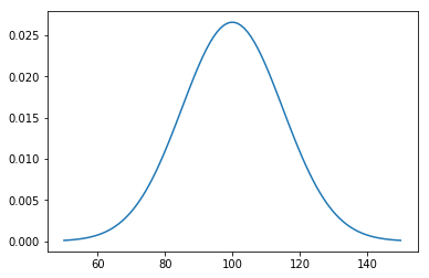
Example: modeling IQ
Suppose IQ is normally distributed with a mean of 0 and a standard deviation of 15.
In [26]:
dist = stats.norm(loc=100, scale=15)
Random variates
In [27]:
dist.rvs(10)
Out[27]:
array([102.95226865,  96.91750482, 104.65750016,  73.69609133,
       101.89198205,  88.0353772 ,  78.79482104,  83.95901608,
        80.87250034, 120.23829691])
In [28]:
xs = np.linspace(50, 150, 100)
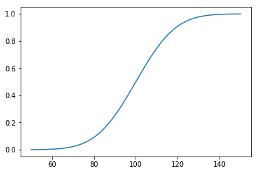
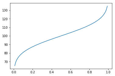
Percentiles
In [31]:
cdf = np.linspace(0, 1, 100)
plt.plot(cdf, dist.ppf(cdf))
pass
In [32]:
data = np.random.normal(110, 15, 100)
Exercises
1. If your IQ is 138, what percentage of the population has a higher IQ?
In [33]:
dist = stats.norm(loc=100, scale=15)
In [34]:
100 * (1 - dist.cdf(138))
Out[34]:
0.564917275556065
Via simulation
In [35]:
n = int(1e6)
samples = dist.rvs(n)
In [36]:
np.sum(samples > 138)/n
Out[36]:
0.005633
2. If your IQ is at the 88th percentile, what is your IQ?
In [37]:
dist.ppf(0.88)
Out[37]:
117.62480188099136
Via simulation
In [38]:
samples = np.sort(samples)
samples[int(0.88*n)]
Out[38]:
117.64535604385766
3. What proportion of the population has IQ between 70 and 90?
In [39]:
dist.cdf(90) - dist.cdf(70)
Out[39]:
0.2297424055987437
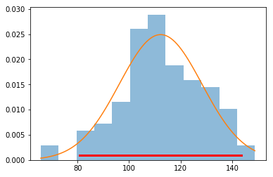
MLE fit and confidence intervals
In [41]:
loc, scale = stats.norm.fit(data)
loc, scale
Out[41]:
(112.25659704843358, 16.021346409851716)
In [42]:
dist = stats.norm(loc, scale)
In [43]:
xs = np.linspace(data.min(), data.max(), 100)
plt.hist(data, 12, histtype='stepfilled', normed=True, alpha=0.5)
plt.plot(xs, dist.pdf(xs))
plt.plot(dist.interval(0.95), [0.001, 0.001], c='r', linewidth=3)
pass
Sampling
Without replication
In [44]:
np.random.choice(range(10), 5, replace=False)
Out[44]:
array([7, 3, 4, 1, 2])
With replication
In [45]:
np.random.choice(range(10), 15)
Out[45]:
array([5, 8, 5, 2, 4, 5, 7, 9, 6, 6, 8, 6, 9, 8, 8])
Example
- How often do we get a run of 5 or more consecutive heads in 100 coin tosses if we repeat the experiment 1000 times?
- What if the coin is biased to generate heads only 40% of the time?
In [46]:
expts = 1000
tosses = 100
We assume that 0 maps to T and 1 to H
In [47]:
xs = np.random.choice([0,1], (expts, tosses))
For biased coin
In [48]:
ys = np.random.choice([0,1], (expts, tosses), p=[0.6, 0.4])
Using a finite state machine
In [49]:
runs = 0
for x in xs:
    m = 0
    for i in x:
        if i == 1:
            m += 1
            if m >=5:
                runs += 1
                break
        else:
            m = 0
runs
Out[49]:
808
Using partitionby
In [50]:
runs = 0
for x in xs:
    parts = tz.partitionby(lambda i: i==1, x)
    for part in parts:
        if part[0] == 1 and len(part) >= 5:
            runs += 1
            break
runs
Out[50]:
808
Using sliding windows
In [51]:
runs = 0
for x in xs:
    for w in tz.sliding_window(5, x):
        if np.sum(w) == 5:
            runs += 1
            break
runs
Out[51]:
808
Using a regular expression
In [52]:
xs = xs.astype('str')
In [53]:
runs = 0
for x in xs:
    if (re.search(r'1{5,}', ''.join(x))):
        runs += 1
runs
Out[53]:
808
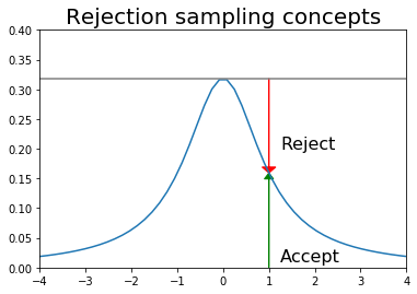
Rejection sampling
Suppose we want random samples from some distribution for which we can calculate the PDF at a point, but lack a direct way to generate random deviates from. One simple idea that is also used in MCMC is rejection sampling - first generate a sample from a distribution from which we can draw samples (e.g. uniform or normal), and then accept or reject this sample with probability some probability (see figure).
Example: Rejection sampling from uniform distribution
We want to draw samples from a Cauchy distribution restricted to (-4, 4). We could choose a more efficient sampling/proposal distribution than the uniform, but this is just to illustrate the concept.
In [54]:
x = np.linspace(-4, 4)

df = 10
dist = stats.cauchy()
upper = dist.pdf(0)
In [55]:
plt.plot(x, dist.pdf(x))
plt.axhline(upper, color='grey')
px = 1.0
plt.arrow(px,0,0,dist.pdf(1.0)-0.01, linewidth=1,
          head_width=0.2, head_length=0.01, fc='g', ec='g')
plt.arrow(px,upper,0,-(upper-dist.pdf(px)-0.01), linewidth=1,
          head_width=0.3, head_length=0.01, fc='r', ec='r')
plt.text(px+.25, 0.2, 'Reject', fontsize=16)
plt.text(px+.25, 0.01, 'Accept', fontsize=16)
plt.axis([-4,4,0,0.4])
plt.title('Rejection sampling concepts', fontsize=20)
pass
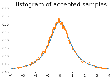
In [56]:
n = 100000
# generate from sampling distribution
u = np.random.uniform(-4, 4, n)
# accept-reject criterion for each point in sampling distribution
r = np.random.uniform(0, upper, n)
# accepted points will come from target (Cauchy) distribution
v = u[r < dist.pdf(u)]

plt.plot(x, dist.pdf(x), linewidth=2)

# Plot scaled histogram
factor = dist.cdf(4) - dist.cdf(-4)
hist, bin_edges = np.histogram(v, bins=100, normed=True)
bin_centers = (bin_edges[:-1] + bin_edges[1:]) / 2.
plt.step(bin_centers, factor*hist, linewidth=2)

plt.axis([-4,4,0,0.4])
plt.title('Histogram of accepted samples', fontsize=20)
pass
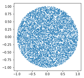
Example: Random samples from the unit circle using rejection sampling
In [57]:
x = np.random.uniform(-1, 1, (10000, 2))
x = x[np.sum(x**2, axis=1) < 1]
plt.scatter(x[:, 0], x[:,1], s=1)
plt.axis('square')
pass