Numbers
In [1]:
%matplotlib inline
In [2]:
import matplotlib.pyplot as plt
In [3]:
import numpy as np
The ndarray: Vectors, matrices and tenosrs
dtype, shape, strides
Vector
In [4]:
x = np.array([1,2,3])
x
Out[4]:
array([1, 2, 3])
In [5]:
type(x)
Out[5]:
numpy.ndarray
In [6]:
x.dtype
Out[6]:
dtype('int64')
In [7]:
x.shape
Out[7]:
(3,)
In [8]:
x.strides
Out[8]:
(8,)
Matrix
In [9]:
x = np.array([[1,2,3], [4,5,6]], dtype=np.int32)
x
Out[9]:
array([[1, 2, 3],
       [4, 5, 6]], dtype=int32)
In [10]:
x.dtype
Out[10]:
dtype('int32')
In [11]:
x.shape
Out[11]:
(2, 3)
In [12]:
x.strides
Out[12]:
(12, 4)
Tensor
In [13]:
x = np.arange(24).reshape((2,3,4))
In [14]:
x
Out[14]:
array([[[ 0,  1,  2,  3],
        [ 4,  5,  6,  7],
        [ 8,  9, 10, 11]],

       [[12, 13, 14, 15],
        [16, 17, 18, 19],
        [20, 21, 22, 23]]])
Creating ndarrays
From a file
In [15]:
%%file numbers.txt
a,b,c # can also skip headers
1,2,3
4,5,6
Overwriting numbers.txt
In [16]:
np.loadtxt('numbers.txt', dtype='int', delimiter=',',
           skiprows=1, comments='#')
Out[16]:
array([[1, 2, 3],
       [4, 5, 6]])
From Python lists or tuples
In [17]:
np.array([
    [1,2,3],
    [4,5,6]
])
Out[17]:
array([[1, 2, 3],
       [4, 5, 6]])
From ranges
arange, linspace, logspace
In [18]:
np.arange(1, 7).reshape((2,3))
Out[18]:
array([[1, 2, 3],
       [4, 5, 6]])
In [19]:
np.linspace(1, 10, 4)
Out[19]:
array([ 1., 4., 7., 10.])
In [20]:
np.logspace(0, 4, 5, dtype='int')
Out[20]:
array([ 1, 10, 100, 1000, 10000])
From a function
fromfunciton
In [21]:
np.fromfunction(lambda i, j: i*3 + j + 1, (2,3))
Out[21]:
array([[ 1.,  2.,  3.],
       [ 4.,  5.,  6.]])
In [22]:
np.fromfunction(lambda i, j: (i-2)**2 + (j-2)**2, (5,5))
Out[22]:
array([[ 8.,  5.,  4.,  5.,  8.],
       [ 5.,  2.,  1.,  2.,  5.],
       [ 4.,  1.,  0.,  1.,  4.],
       [ 5.,  2.,  1.,  2.,  5.],
       [ 8.,  5.,  4.,  5.,  8.]])
In [23]:
np.fromfunction(lambda i, j: np.where(i<j, 1, np.where(i==j,0, -1)), (5,5))
Out[23]:
array([[ 0,  1,  1,  1,  1],
       [-1,  0,  1,  1,  1],
       [-1, -1,  0,  1,  1],
       [-1, -1, -1,  0,  1],
       [-1, -1, -1, -1,  0]])
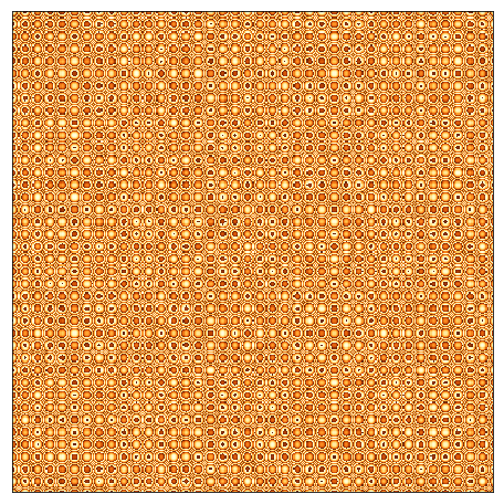
Adapted from Circle Squared
In [24]:
xs = np.fromfunction(lambda i, j:  0.27**2*(i**2 + j**2) % 1.5,
                     (400, 400),)
plt.figure(figsize=(8,8))
plt.imshow(xs, interpolation='nearest', cmap=plt.cm.YlOrBr)
plt.xticks([])
plt.yticks([])
pass
From special construcotrs
zeoros, ones, eye
In [25]:
np.zeros((2,3))
Out[25]:
array([[ 0.,  0.,  0.],
       [ 0.,  0.,  0.]])
In [26]:
np.ones((2,3))
Out[26]:
array([[ 1.,  1.,  1.],
       [ 1.,  1.,  1.]])
In [27]:
np.eye(3)
Out[27]:
array([[ 1.,  0.,  0.],
       [ 0.,  1.,  0.],
       [ 0.,  0.,  1.]])
In [28]:
np.eye(3, 4)
Out[28]:
array([[ 1.,  0.,  0.,  0.],
       [ 0.,  1.,  0.,  0.],
       [ 0.,  0.,  1.,  0.]])
In [29]:
np.eye(4, k=-1)
Out[29]:
array([[ 0.,  0.,  0.,  0.],
       [ 1.,  0.,  0.,  0.],
       [ 0.,  1.,  0.,  0.],
       [ 0.,  0.,  1.,  0.]])
From random variables
Convenience functions
rand, randn
In [30]:
np.random.rand(2,3)
Out[30]:
array([[ 0.04737547,  0.82228651,  0.22224204],
       [ 0.96886745,  0.54149529,  0.94853004]])
In [31]:
np.random.randn(2,3)
Out[31]:
array([[-0.80516331,  0.9086527 , -1.21134755],
       [-0.08444392,  1.00515737,  0.94762797]])
Distributions
uniform, normal, randint, poisson, multinomial, multivariate_ normal
In [32]:
np.random.uniform(0, 1, (2,3))
Out[32]:
array([[ 0.12880127,  0.32643222,  0.52082391],
       [ 0.35404701,  0.54964578,  0.456206  ]])
In [33]:
np.random.normal(0, 1, (2,3))
Out[33]:
array([[ 0.8195548 ,  0.43940477, -0.24901744],
       [ 2.6248388 ,  0.16150201,  0.12905971]])
In [34]:
np.random.randint(0, 10, (4,5))
Out[34]:
array([[5, 0, 2, 3, 9],
       [8, 5, 1, 1, 9],
       [5, 5, 2, 0, 2],
       [2, 0, 5, 7, 4]])
In [35]:
np.random.poisson(10, (4,5))
Out[35]:
array([[ 8,  9, 17,  8, 15],
       [ 8,  9, 12, 12, 11],
       [ 6,  8, 10, 13,  6],
       [ 7, 12,  8, 16,  8]])
In [36]:
np.random.multinomial(n=5, pvals=np.ones(5)/5, size=8)
Out[36]:
array([[2, 0, 0, 2, 1],
       [4, 0, 0, 1, 0],
       [3, 0, 0, 1, 1],
       [1, 1, 1, 1, 1],
       [0, 1, 2, 1, 1],
       [1, 1, 2, 1, 0],
       [2, 0, 1, 1, 1],
       [0, 1, 1, 1, 2]])
In [37]:
np.random.multivariate_normal(mean=[10,20,30], cov=np.eye(3), size=4)
Out[37]:
array([[  9.34907429,  20.28742704,  31.20954084],
       [ 10.61473257,  19.60538925,  29.09199082],
       [  9.10517086,  19.82157961,  28.57954932],
       [  8.35947889,  22.60010629,  29.05471801]])
Indexing
In [38]:
x = np.arange(20).reshape((4,5))
x
Out[38]:
array([[ 0,  1,  2,  3,  4],
       [ 5,  6,  7,  8,  9],
       [10, 11, 12, 13, 14],
       [15, 16, 17, 18, 19]])
Using slices
In [41]:
x[1,:]
Out[41]:
array([5, 6, 7, 8, 9])
In [42]:
x[:,1]
Out[42]:
array([ 1, 6, 11, 16])
In [43]:
x[1:3,1:3]
Out[43]:
array([[ 6,  7],
       [11, 12]])
Extrcting blocks with arbitrary row and column lists (fancy indexing)
np.ix_
In [45]:
x[:, [0,3]]
Out[45]:
array([[ 0,  3],
       [ 5,  8],
       [10, 13],
       [15, 18]])
Warning: Fancy indexing can only be used for 1 dimension.
In [46]:
x[[0,2],[0,3]]
Out[46]:
array([ 0, 13])
Use the helper np.ix_ to extract arbitrary blocks.
In [47]:
x[np.ix_([0,2], [0,3])]
Out[47]:
array([[ 0,  3],
       [10, 13]])
A slice is a view, not a copy
In [48]:
x
Out[48]:
array([[ 0,  1,  2,  3,  4],
       [ 5,  6,  7,  8,  9],
       [10, 11, 12, 13, 14],
       [15, 16, 17, 18, 19]])
In [49]:
y = x[1:-1, 1:-1]
y
Out[49]:
array([[ 6,  7,  8],
       [11, 12, 13]])
In [50]:
y *= 10
In [51]:
y
Out[51]:
array([[ 60,  70,  80],
       [110, 120, 130]])
In [52]:
x
Out[52]:
array([[  0,   1,   2,   3,   4],
       [  5,  60,  70,  80,   9],
       [ 10, 110, 120, 130,  14],
       [ 15,  16,  17,  18,  19]])
Use the copy method to convert a view to a copy
In [53]:
z = x[1:-1, 1:-1].copy()
In [54]:
z
Out[54]:
array([[ 60,  70,  80],
       [110, 120, 130]])
In [55]:
z[:] = 0
In [56]:
z
Out[56]:
array([[0, 0, 0],
       [0, 0, 0]])
In [57]:
x
Out[57]:
array([[  0,   1,   2,   3,   4],
       [  5,  60,  70,  80,   9],
       [ 10, 110, 120, 130,  14],
       [ 15,  16,  17,  18,  19]])
Boolean indexing
In [58]:
x[x % 2 == 0]
Out[58]:
array([ 0, 2, 4, 60, 70, 80, 10, 110, 120, 130, 14, 16, 18])
In [59]:
x [x > 3]
Out[59]:
array([  4,   5,  60,  70,  80,   9,  10, 110, 120, 130,  14,  15,  16,
        17,  18,  19])
Functions that return indexes
In [60]:
idx = np.nonzero(x)
idx
Out[60]:
(array([0, 0, 0, 0, 1, 1, 1, 1, 1, 2, 2, 2, 2, 2, 3, 3, 3, 3, 3]),
 array([1, 2, 3, 4, 0, 1, 2, 3, 4, 0, 1, 2, 3, 4, 0, 1, 2, 3, 4]))
In [61]:
x[idx]
Out[61]:
array([  1,   2,   3,   4,   5,  60,  70,  80,   9,  10, 110, 120, 130,
        14,  15,  16,  17,  18,  19])
In [62]:
idx = np.where(x > 3)
idx
Out[62]:
(array([0, 1, 1, 1, 1, 1, 2, 2, 2, 2, 2, 3, 3, 3, 3, 3]),
 array([4, 0, 1, 2, 3, 4, 0, 1, 2, 3, 4, 0, 1, 2, 3, 4]))
In [63]:
x[idx]
Out[63]:
array([  4,   5,  60,  70,  80,   9,  10, 110, 120, 130,  14,  15,  16,
        17,  18,  19])
Margins and the axis argument
In [64]:
x
Out[64]:
array([[  0,   1,   2,   3,   4],
       [  5,  60,  70,  80,   9],
       [ 10, 110, 120, 130,  14],
       [ 15,  16,  17,  18,  19]])
The 0th axis has 4 items, the 1st axis has 5 items.
In [65]:
x.shape
Out[65]:
(4, 5)
In [66]:
x.mean()
Out[66]:
35.149999999999999
Marginalizing out the 0th axis = column summaries
In [67]:
x.mean(axis=0)
Out[67]:
array([ 7.5 , 46.75, 52.25, 57.75, 11.5 ])
Marginalizing out the 1st axis = row summaries
In [68]:
x.mean(axis=1)
Out[68]:
array([ 2. , 44.8, 76.8, 17. ])
Note marginalizing out the last axis is a common default.
In [69]:
x.mean(axis=-1)
Out[69]:
array([ 2. , 44.8, 76.8, 17. ])
Marginalization works for higher dimensions in the same way
In [70]:
x = np.random.random((2,3,4))
x
Out[70]:
array([[[ 0.25091919,  0.97511897,  0.6520031 ,  0.56832053],
        [ 0.97444408,  0.72376855,  0.15067567,  0.10752009],
        [ 0.20627991,  0.0234196 ,  0.70143528,  0.87408988]],

       [[ 0.95505841,  0.79364654,  0.76668484,  0.47971008],
        [ 0.34780788,  0.44169709,  0.63645331,  0.96215426],
        [ 0.92889169,  0.52710155,  0.22280321,  0.04262088]]])
In [71]:
x.shape
Out[71]:
(2, 3, 4)
In [72]:
x.mean(axis=0).shape
Out[72]:
(3, 4)
In [73]:
x.mean(axis=1).shape
Out[73]:
(2, 4)
In [74]:
x.mean(axis=2).shape
Out[74]:
(2, 3)
In [75]:
x.mean(axis=(0,1)).shape
Out[75]:
(4,)
In [76]:
x.mean(axis=(0,2)).shape
Out[76]:
(3,)
In [77]:
x.mean(axis=(1,2)).shape
Out[77]:
(2,)
Broadcasting
In [78]:
x1 = np.arange(12)
In [79]:
x1
Out[79]:
array([ 0, 1, 2, 3, 4, 5, 6, 7, 8, 9, 10, 11])
In [80]:
x1 * 10
Out[80]:
array([ 0, 10, 20, 30, 40, 50, 60, 70, 80, 90, 100, 110])
In [81]:
x2 = np.random.randint(0,10,(3,4))
In [82]:
x2
Out[82]:
array([[3, 0, 1, 2],
       [2, 4, 0, 7],
       [9, 9, 3, 0]])
In [83]:
x2 * 10
Out[83]:
array([[30,  0, 10, 20],
       [20, 40,  0, 70],
       [90, 90, 30,  0]])
In [84]:
x2.shape
Out[84]:
(3, 4)
Column-wise broadcasting
In [85]:
mu = np.mean(x2, axis=0)
mu.shape
Out[85]:
(4,)
In [86]:
x2 - mu
Out[86]:
array([[-1.66666667, -4.33333333, -0.33333333, -1.        ],
       [-2.66666667, -0.33333333, -1.33333333,  4.        ],
       [ 4.33333333,  4.66666667,  1.66666667, -3.        ]])
In [87]:
(x2 - mu).mean(axis=0)
Out[87]:
array([ -2.96059473e-16,   2.96059473e-16,   7.40148683e-17,
         0.00000000e+00])
Row wise broadcasting
In [88]:
mu = np.mean(x2, axis=1)
mu.shape
Out[88]:
(3,)
In [89]:
try:
    x2 - mu
except ValueError as e:
    print(e)
operands could not be broadcast together with shapes (3,4) (3,)
We can add a “dummy” axis using None or np.newaxis
In [90]:
mu[:, None].shape
Out[90]:
(3, 1)
In [91]:
x2 - mu[:, None]
Out[91]:
array([[ 1.5 , -1.5 , -0.5 ,  0.5 ],
       [-1.25,  0.75, -3.25,  3.75],
       [ 3.75,  3.75, -2.25, -5.25]])
In [92]:
x2 - mu[:, np.newaxis]
Out[92]:
array([[ 1.5 , -1.5 , -0.5 ,  0.5 ],
       [-1.25,  0.75, -3.25,  3.75],
       [ 3.75,  3.75, -2.25, -5.25]])
In [93]:
np.mean(x2 - mu[:, None], axis=1)
Out[93]:
array([ 0., 0., 0.])
Reshaping works too
In [94]:
x2 - mu.reshape((-1,1))
Out[94]:
array([[ 1.5 , -1.5 , -0.5 ,  0.5 ],
       [-1.25,  0.75, -3.25,  3.75],
       [ 3.75,  3.75, -2.25, -5.25]])
Broadcasting examples
Creating a 12 by 12 multiplication table
In [95]:
x = np.arange(1, 13)
x[:,None] * x[None,:]
Out[95]:
array([[  1,   2,   3,   4,   5,   6,   7,   8,   9,  10,  11,  12],
       [  2,   4,   6,   8,  10,  12,  14,  16,  18,  20,  22,  24],
       [  3,   6,   9,  12,  15,  18,  21,  24,  27,  30,  33,  36],
       [  4,   8,  12,  16,  20,  24,  28,  32,  36,  40,  44,  48],
       [  5,  10,  15,  20,  25,  30,  35,  40,  45,  50,  55,  60],
       [  6,  12,  18,  24,  30,  36,  42,  48,  54,  60,  66,  72],
       [  7,  14,  21,  28,  35,  42,  49,  56,  63,  70,  77,  84],
       [  8,  16,  24,  32,  40,  48,  56,  64,  72,  80,  88,  96],
       [  9,  18,  27,  36,  45,  54,  63,  72,  81,  90,  99, 108],
       [ 10,  20,  30,  40,  50,  60,  70,  80,  90, 100, 110, 120],
       [ 11,  22,  33,  44,  55,  66,  77,  88,  99, 110, 121, 132],
       [ 12,  24,  36,  48,  60,  72,  84,  96, 108, 120, 132, 144]])
Scaling to have zero mean and unit standard devation for each feature.
In [96]:
x = np.random.normal(10, 5,(3,4))
x
Out[96]:
array([[  7.65396872,   8.74106757,   7.26659687,   9.68096491],
       [  9.27132075,   7.89349589,   9.47813473,   7.04088855],
       [ 13.78187972,   7.39243968,  10.90034325,   4.27477767]])
Standardize column-wise
In [97]:
(x - x.mean(axis=0))/x.std(axis=0)
Out[97]:
array([[-0.99566783,  1.31524702, -1.30321654,  1.21511731],
       [-0.37192708, -0.20751913,  0.17598238,  0.01903327],
       [ 1.36759491, -1.10772789,  1.12723416, -1.23415058]])
Standardize row-wise
In [98]:
(x - x.mean(axis=1)[:, None])/x.std(axis=1)[:, None]
Out[98]:
array([[-0.72037796,  0.42843253, -1.12973985,  1.42168528],
       [ 0.84786879, -0.52591836,  1.0540767 , -1.37602714],
       [ 1.31012381, -0.47301018,  0.50595856, -1.34307219]])
Combining ndarrays
In [99]:
x1 = np.zeros((3,4))
x2 = np.ones((3,5))
x3 = np.eye(4)
In [100]:
x1
Out[100]:
array([[ 0.,  0.,  0.,  0.],
       [ 0.,  0.,  0.,  0.],
       [ 0.,  0.,  0.,  0.]])
In [101]:
x2
Out[101]:
array([[ 1.,  1.,  1.,  1.,  1.],
       [ 1.,  1.,  1.,  1.,  1.],
       [ 1.,  1.,  1.,  1.,  1.]])
In [102]:
x3
Out[102]:
array([[ 1.,  0.,  0.,  0.],
       [ 0.,  1.,  0.,  0.],
       [ 0.,  0.,  1.,  0.],
       [ 0.,  0.,  0.,  1.]])
Binding rows when number of columns is the same
In [103]:
np.r_[x1, x3]
Out[103]:
array([[ 0.,  0.,  0.,  0.],
       [ 0.,  0.,  0.,  0.],
       [ 0.,  0.,  0.,  0.],
       [ 1.,  0.,  0.,  0.],
       [ 0.,  1.,  0.,  0.],
       [ 0.,  0.,  1.,  0.],
       [ 0.,  0.,  0.,  1.]])
Binding columns when number of rows is the same
In [104]:
np.c_[x1, x2]
Out[104]:
array([[ 0.,  0.,  0.,  0.,  1.,  1.,  1.,  1.,  1.],
       [ 0.,  0.,  0.,  0.,  1.,  1.,  1.,  1.,  1.],
       [ 0.,  0.,  0.,  0.,  1.,  1.,  1.,  1.,  1.]])
You can combine more than 2 at a time
In [105]:
np.c_[x1, x2, x1]
Out[105]:
array([[ 0.,  0.,  0.,  0.,  1.,  1.,  1.,  1.,  1.,  0.,  0.,  0.,  0.],
       [ 0.,  0.,  0.,  0.,  1.,  1.,  1.,  1.,  1.,  0.,  0.,  0.,  0.],
       [ 0.,  0.,  0.,  0.,  1.,  1.,  1.,  1.,  1.,  0.,  0.,  0.,  0.]])
Stacking
In [106]:
np.vstack([x1, x3])
Out[106]:
array([[ 0.,  0.,  0.,  0.],
       [ 0.,  0.,  0.,  0.],
       [ 0.,  0.,  0.,  0.],
       [ 1.,  0.,  0.,  0.],
       [ 0.,  1.,  0.,  0.],
       [ 0.,  0.,  1.,  0.],
       [ 0.,  0.,  0.,  1.]])
In [107]:
np.hstack([x1, x2])
Out[107]:
array([[ 0.,  0.,  0.,  0.,  1.,  1.,  1.,  1.,  1.],
       [ 0.,  0.,  0.,  0.,  1.,  1.,  1.,  1.,  1.],
       [ 0.,  0.,  0.,  0.,  1.,  1.,  1.,  1.,  1.]])
In [108]:
np.dstack([x2, 2*x2, 3*x2])
Out[108]:
array([[[ 1.,  2.,  3.],
        [ 1.,  2.,  3.],
        [ 1.,  2.,  3.],
        [ 1.,  2.,  3.],
        [ 1.,  2.,  3.]],

       [[ 1.,  2.,  3.],
        [ 1.,  2.,  3.],
        [ 1.,  2.,  3.],
        [ 1.,  2.,  3.],
        [ 1.,  2.,  3.]],

       [[ 1.,  2.,  3.],
        [ 1.,  2.,  3.],
        [ 1.,  2.,  3.],
        [ 1.,  2.,  3.],
        [ 1.,  2.,  3.]]])
Generic stack with axis argument
In [109]:
np.stack([x2, 2*x2, 3*x2], axis=0)
Out[109]:
array([[[ 1.,  1.,  1.,  1.,  1.],
        [ 1.,  1.,  1.,  1.,  1.],
        [ 1.,  1.,  1.,  1.,  1.]],

       [[ 2.,  2.,  2.,  2.,  2.],
        [ 2.,  2.,  2.,  2.,  2.],
        [ 2.,  2.,  2.,  2.,  2.]],

       [[ 3.,  3.,  3.,  3.,  3.],
        [ 3.,  3.,  3.,  3.,  3.],
        [ 3.,  3.,  3.,  3.,  3.]]])
In [110]:
np.stack([x2, 2*x2, 3*x2], axis=1)
Out[110]:
array([[[ 1.,  1.,  1.,  1.,  1.],
        [ 2.,  2.,  2.,  2.,  2.],
        [ 3.,  3.,  3.,  3.,  3.]],

       [[ 1.,  1.,  1.,  1.,  1.],
        [ 2.,  2.,  2.,  2.,  2.],
        [ 3.,  3.,  3.,  3.,  3.]],

       [[ 1.,  1.,  1.,  1.,  1.],
        [ 2.,  2.,  2.,  2.,  2.],
        [ 3.,  3.,  3.,  3.,  3.]]])
In [111]:
np.stack([x2, 2*x2, 3*x2], axis=2)
Out[111]:
array([[[ 1.,  2.,  3.],
        [ 1.,  2.,  3.],
        [ 1.,  2.,  3.],
        [ 1.,  2.,  3.],
        [ 1.,  2.,  3.]],

       [[ 1.,  2.,  3.],
        [ 1.,  2.,  3.],
        [ 1.,  2.,  3.],
        [ 1.,  2.,  3.],
        [ 1.,  2.,  3.]],

       [[ 1.,  2.,  3.],
        [ 1.,  2.,  3.],
        [ 1.,  2.,  3.],
        [ 1.,  2.,  3.],
        [ 1.,  2.,  3.]]])
Repetition and tiling
For a vector
In [112]:
x = np.array([1,2,3])
In [113]:
np.repeat(x, 3)
Out[113]:
array([1, 1, 1, 2, 2, 2, 3, 3, 3])
In [114]:
np.tile(x, 3)
Out[114]:
array([1, 2, 3, 1, 2, 3, 1, 2, 3])
For a matrix
In [115]:
x = np.arange(6).reshape((2,3))
x
Out[115]:
array([[0, 1, 2],
       [3, 4, 5]])
In [116]:
np.repeat(x, 3)
Out[116]:
array([0, 0, 0, 1, 1, 1, 2, 2, 2, 3, 3, 3, 4, 4, 4, 5, 5, 5])
In [117]:
np.repeat(x, 3, axis=0)
Out[117]:
array([[0, 1, 2],
       [0, 1, 2],
       [0, 1, 2],
       [3, 4, 5],
       [3, 4, 5],
       [3, 4, 5]])
In [118]:
np.repeat(x, 3, axis=1)
Out[118]:
array([[0, 0, 0, 1, 1, 1, 2, 2, 2],
       [3, 3, 3, 4, 4, 4, 5, 5, 5]])
In [119]:
np.tile(x, 3)
Out[119]:
array([[0, 1, 2, 0, 1, 2, 0, 1, 2],
       [3, 4, 5, 3, 4, 5, 3, 4, 5]])
Splitting ndarrays
In [120]:
x = np.arange(32).reshape((4,8))
In [121]:
x
Out[121]:
array([[ 0,  1,  2,  3,  4,  5,  6,  7],
       [ 8,  9, 10, 11, 12, 13, 14, 15],
       [16, 17, 18, 19, 20, 21, 22, 23],
       [24, 25, 26, 27, 28, 29, 30, 31]])
In [122]:
np.split(x, 4)
Out[122]:
[array([[0, 1, 2, 3, 4, 5, 6, 7]]),
 array([[ 8,  9, 10, 11, 12, 13, 14, 15]]),
 array([[16, 17, 18, 19, 20, 21, 22, 23]]),
 array([[24, 25, 26, 27, 28, 29, 30, 31]])]
In [123]:
np.split(x, 4, axis=1)
Out[123]:
[array([[ 0,  1],
        [ 8,  9],
        [16, 17],
        [24, 25]]), array([[ 2,  3],
        [10, 11],
        [18, 19],
        [26, 27]]), array([[ 4,  5],
        [12, 13],
        [20, 21],
        [28, 29]]), array([[ 6,  7],
        [14, 15],
        [22, 23],
        [30, 31]])]
Vectorization
Example 1
The operators and functions (ufuncs) in Python are vectorized, and will
work element-wise over all entries in an ndarray.
In [124]:
xs = np.zeros(10, dtype='int')
for i in range(10):
    xs[i] = i**2
xs
Out[124]:
array([ 0, 1, 4, 9, 16, 25, 36, 49, 64, 81])
In [125]:
xs = np.arange(10)**2
xs
Out[125]:
array([ 0, 1, 4, 9, 16, 25, 36, 49, 64, 81])
Using ufuncs
In [126]:
np.sqrt(xs)
Out[126]:
array([ 0., 1., 2., 3., 4., 5., 6., 7., 8., 9.])
In [127]:
np.log1p(xs)
Out[127]:
array([ 0.        ,  0.69314718,  1.60943791,  2.30258509,  2.83321334,
        3.25809654,  3.61091791,  3.91202301,  4.17438727,  4.40671925])
Example 2
In [128]:
n = 10

xs = np.random.rand(n)
ys = np.random.rand(n)

s = 0
for i in range(n):
    s += xs[i] * ys[i]
s
Out[128]:
2.6868481407430282
In [129]:
np.dot(xs, ys)
Out[129]:
2.6868481407430282
In [130]:
xs @ ys
Out[130]:
2.6868481407430282
Example 3
In [131]:
m = 3
n = 2

alpha = np.random.rand(1)
betas = np.random.rand(n,1)
xs = np.random.rand(m,n)
In [132]:
alpha
Out[132]:
array([ 0.05007867])
In [133]:
betas
Out[133]:
array([[ 0.06399532],
       [ 0.37993848]])
In [134]:
xs
Out[134]:
array([[ 0.79258489,  0.20951971],
       [ 0.89978267,  0.044122  ],
       [ 0.34222118,  0.06629664]])
Using loops
In [135]:
ys = np.zeros((m,1))
for i in range(m):
    ys[i] = alpha
    for j in range(n):
        ys[i] += betas[j] * xs[i,j]
ys
Out[135]:
array([[ 0.180405  ],
       [ 0.1244242 ],
       [ 0.09716787]])
Removing inner loop
In [136]:
ys = np.zeros((m,1))
for i in range(m):
    ys[i] = alpha + xs[i,:].T @ betas
ys
Out[136]:
array([[ 0.180405  ],
       [ 0.1244242 ],
       [ 0.09716787]])
Removing all loops
In [137]:
ys = alpha + xs @ betas
ys
Out[137]:
array([[ 0.180405  ],
       [ 0.1244242 ],
       [ 0.09716787]])
Alternative approach
The calculaiton with explicit intercepts and coefficients is common in deep learning, where \(\alpha\) is called the bias (\(b\)) and \(\beta\) are called the weights (\(w\)), and each equation is \(y[i] = b + w[i]*x[i]\).
It is common in statisiics to use an augmented matrix in which the first column is all ones, so that all that is needed is a single matrix multiplicaiotn.
In [138]:
X = np.c_[np.ones(m), xs]
X
Out[138]:
array([[ 1.        ,  0.79258489,  0.20951971],
       [ 1.        ,  0.89978267,  0.044122  ],
       [ 1.        ,  0.34222118,  0.06629664]])
In [139]:
alpha
Out[139]:
array([ 0.05007867])
In [140]:
betas
Out[140]:
array([[ 0.06399532],
       [ 0.37993848]])
In [141]:
betas_ = np.concatenate([[alpha], betas])
betas_
Out[141]:
array([[ 0.05007867],
       [ 0.06399532],
       [ 0.37993848]])
In [142]:
ys = X @ betas_
ys
Out[142]:
array([[ 0.180405  ],
       [ 0.1244242 ],
       [ 0.09716787]])
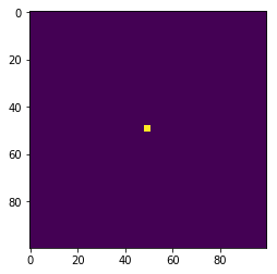
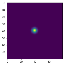
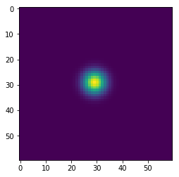
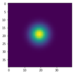
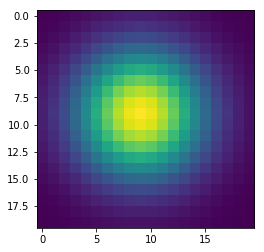
Simulating diffusion
In [143]:
w = 100
h = 100
x = np.zeros((w+2,h+2), dtype='float')
x[(w//2-1):(w//2+2), (h//2-1):(h//2+2)] = 1

wts = np.ones(5)/5

for i in range(41):
    if i % 10 == 0:
        plt.figure()
        plt.imshow(x[1:-1, 1:-1], interpolation='nearest')

    center = x[1:-1, 1:-1]
    left = x[:-2, 1:-1]
    right = x[2:, 1:-1]
    bottom = x[1:-1, :-2]
    top = x[1:-1, 2:]
    nbrs = np.dstack([center, left, right, bottom, top])
    x = np.sum(wts * nbrs, axis=-1)