%matplotlib inline
%load_ext Cython

import math
import numpy as np
import matplotlib.pyplot as plt
import seaborn as sns
from sklearn.datasets import make_blobs
from numba import jit, vectorize, float64, int64

sns.set_context('notebook', font_scale=1.5)

Lab10: Making Python faster

This homework provides practice in making Python code faster. Note that we start with functions that already use idiomatic numpy (which are about two orders of magnitude faster than the pure Python versions).

Functions to optimize

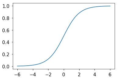
def logistic(x):
    """Logistic function."""
    return np.exp(x)/(1 + np.exp(x))

def gd(X, y, beta, alpha, niter):
    """Gradient descent algorihtm."""
    n, p = X.shape
    Xt = X.T
    for i in range(niter):
        y_pred = logistic(X @ beta)
        epsilon = y - y_pred
        grad = Xt @ epsilon / n
        beta += alpha * grad
    return beta

x = np.linspace(-6, 6, 100)
plt.plot(x, logistic(x))
pass

Data set for classification

n = 10000
p = 2
X, y = make_blobs(n_samples=n, n_features=p, centers=2, cluster_std=1.05, random_state=23)
X = np.c_[np.ones(len(X)), X]
y = y.astype('float')

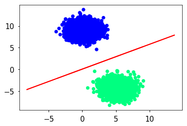
Using gradient descent for classification by logistic regression

# initial parameters
niter = 1000
α = 0.01
β = np.zeros(p+1)

# call gradient descent
β = gd(X, y, β, α, niter)

# assign labels to points based on prediction
y_pred = logistic(X @ β)
labels = y_pred > 0.5

# calculate separating plane
sep = (-β[0] - β[1] * X)/β[2]

plt.scatter(X[:, 1], X[:, 2], c=labels, cmap='winter')
plt.plot(X, sep, 'r-')
pass

1. Rewrite the logistic function so it only makes one np.exp call. Compare the time of both versions with the input x given below using the @timeit magic. (10 points)

np.random.seed(123)
n = int(1e7)
x = np.random.normal(0, 1, n)

2. (20 points) Use numba to compile the gradient descent function.

• Use the @vectorize decorator to create a ufunc version of the logistic function and call this logistic_numba_cpu with function signatures of float64(float64). Create another function called logistic_numba_parallel by giving an extra argument to the decorator of target=parallel (5 points)
• For each function, check that the answers are the same as with the original logistic function using np.testing.assert_array_almost_equal. Use %timeit to compare the three logistic functions (5 points)
• Now use @jit to create a JIT_compiled version of the logistic and gd functions, calling them logistic_numba and gd_numba. Provide appropriate function signatures to the decorator in each case. (5 points)
• Compare the two gradient descent functions gd and gd_numba for correctness and performance. (5 points)

3. (30 points) Use cython to compile the gradient descent function.

• Cythonize the logistic function as logistic_cython. Use the --annotate argument to the cython magic function to find slow regions. Compare accuracy and performance. The final performance should be comparable to the numba cpu version. (10 points)
• Now cythonize the gd function as gd_cython. This function should use of the cythonized logistic_cython as a C function call. Compare accuracy and performance. The final performance should be comparable to the numba cpu version. (20 points)

Hints:

• Give static types to all variables
• Know how to use def, cdef and cpdef
• Use Typed MemoryViews
• Find out how to transpose a Typed MemoryView to store the transpose of X
• Typed MemoryVeiws are not numpy arrays - you often have to write explicit loops to operate on them
• Use the cython boundscheck, wraparound, and cdivision operators

4. (40 points) Wrapping modules in C++.

Rewrite the logistic and gd functions in C++, using pybind11 to create Python wrappers. Compare accuracy and performance as usual. Replicate the plotted example using the C++ wrapped functions for logistic and gd

• Writing a vectorized logistic function callable from both C++ and Python (10 points)
• Writing the gd function callable from Python (25 points)
• Checking accuracy, benchmarking and creating diagnostic plots (5 points)

Hints:

• Use the C++ Eigen library to do vector and matrix operations (include path is ../notebooks/eigen3)
• When calling the exponential function, you have to use exp(m.array()) instead of exp(m) if you use an Eigen dynamic template.
• Use cppimport to simplify the wrapping for Python
• See `pybind11 docs <http://pybind11.readthedocs.io/en/latest/index.html>`__
• See my examples for help